WIXLIB

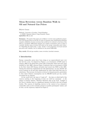
Mean Reversion versus Random Walk inOil and Natural Gas PricesHélyette GemanBirkbeck, University of London, United Kingdom& ESSEC Business School, Cergy-Pontoise, Francehgeman@ems.bbk.ac.ukSummary. The goals of the paper are as follows: i) review some qualitative properties of oil and gas prices in the last 15 years; ii) propose some mathematical elementstowards a definition of mean reversion that would not be reduced to the form of thedrift in a stochastic differential equation; iii) conduct econometric tests in order toconclude whether mean reversion still exists in the energy commodity price behavior. Regarding the third point, a clear “break” in the properties of oil and naturalgas prices and volatility can be exhibited in the period 2000-2001.Key words: Oil and gas markets; mean reversion; invariant measure.1 IntroductionEnergy commodity prices have been rising at an unprecedented pace overthe last five years. As depicted in Figure 1, an investment of 100 made inJanuary 2002 in the global Dow Jones-AIG Commodity Index had more thandoubled by July 2006, whereas Figure 2 indicates that an investment of 100in the Dow Jones-AIG Energy sub-index had turned into 500 in July 2005.Among the numerous explanations for this phenomenon, we may identify thesevere tensions on oil and their implications for other fossil fuels that may besubstitutes. The increase of oil prices is driven by demand growth, particularlyin Asia where Chinese consumption rose by 900,000 barrels per day, mostlyaccounted for by imports.At the world level, the issue of “peak oil” – the date at which half of thereserves existing at the beginning of time are (will be) consumed – is thesubject of intense debates. Matthew Simmons asks in his book, Twilight inthe Desert, whether there is a significant amount of oil left in the soil of SaudiArabia. The concern of depleting reserves in the context of an exhaustivecommodity such as oil is certainly present on market participants’ minds, andin turn, on the trajectory depicted in Figure 2.

228Hélyette GemanFig. 1. Dow Jones-AIG Total Return Index over the period Jan 2002–July 2006.Fig. 2. Dow Jones-AIG Energy Sub-Index over the period Jan 2000–July 2005.

Mean Reversion versus Random Walk in Oil and Natural Gas Prices229Fig. 3. Goldman Sachs Commodity Index Total Return and Dow Jones-AIG Commodity Index total return over the period Feb 1991–Dec 1999.The financial literature on commodity price modeling started with the pioneering paper by Gibson and Schwartz [7]. In the spirit of the Black-ScholesMerton [2] formula, they use a geometric Brownian motion for oil spot prices.Given the behavior of commodity prices during the 1990s depicted in Figure 3 by the two major commodity indexes, [10] introduces a mean-revertingdrift in the stochastic differential equation driving oil price dynamics; [14], [4],[12] keep this mean-reversion representation for oil, electricity and bituminouscoal.The goal of this paper is to revisit the modelling of oil and natural gasprices in the light of the trajectories observed in the recent past (see Figure2), as well as the definition of mean reversion from a general mathematicalperspective. Note that this issue matters also for key quantities in finance suchas stochastic volatility. Fouque, Papanicolaou and Sircar [5] are interested inthe property of clustering exhibited by the volatility of asset prices. Theirview is that volatility is ‘bursty’ in nature, and burstiness is closely relatedto mean reversion, since a bursty process is returning to its mean (at a speedthat depends on the length of the burst period).

230Hélyette Geman2 Some Elements on Mean Reversion in Diffusion from aMathematical PerspectiveThe long-term behavior of continuous time Markov processes has been thesubject of much attention, starting with the work of Has’minskii [8]. Accordingly, the long-term evolution of the price of an exhaustible commodity, suchas oil or copper, is a topic of major concern in finance, given the world geopolitical and economic consequences of this issue. In what follows, (Xt ) willessentially have the economic interpretation of a log-price. We start with aprocess (Xt ) defined as solution of a stochastic differential equationdXt b (Xt ) dt σ (Xt ) dWt ,where (Wt ) is a standard Brownian motion on a probability space (Ω, F, P)describing the randomness of the economy. We know from Itô that if b andσ are Lipschitz, there exists a unique solution to the equation. If only b isLipschitz and σ Holder of coefficient 12 , we still have existence and uniquenessof the solution. In both cases, the process (Xt ) will be Markov and the driftb (Xt ) will contain the representation of the trend perceived at date t for futurespot prices.Given a process (Xt ), we are in finance particularly interested in the possible existence of a distribution for X0 such that, for any positive t, Xt hasthe same distribution. This distribution, if it exists, may be viewed as anequilibrium state for the process. We now recall the definition of an invariant probability measure for a Markov process (Xt )t 0 , whose semi-group isdenoted (Pt )t 0 and satisfies the property that, for any bounded measurablefunction, Pt f (x) E [f (Xt )].Definition 1. (i) A measure µ is said to be invariant for the process (Xt ) ifand only ifZZµ (dx) Pt f (x) µ (dx) f (x) ,for any bounded function f . (ii) µ is invariant for (Xt ) if and only if µPt µ.Equivalently, the law of (Xt u )u 0 is independent of t if we start at date 0with the measure µ.Proposition 1. The existence of an invariant measure implies that the process (Xt ) is stationary. If (Xt ) admits a limit law independent of its initialstate, then this limit law is an invariant measure.Proof. The first part of the proposition is nothing but Rone of the two formsof the definition above. Now suppose E [f (Xt )] t µ (dy) f (y), for anybounded function f . ThenZEX [f (Xt s )] EX [PS f (Xt )] t µ (dy) f (y) .Hence, µPS µ, and µ is invariant.ut

Mean Reversion versus Random Walk in Oil and Natural Gas Prices231Proposition 2. 1. The Ornstein-Uhlenbeck process admits a finite invariantmeasure, and this measure is Gaussian.2. The Cox-Ingersoll-Ross (or square-root) process also has a finite invariantmeasure.3. The arithmetic Brownian motion (like all Lévy processes) admits theLebesgue measure as an invariant measure, hence, not finite.4. A (squared) Bessel process exhibits the same property, namely an infiniteinvariant measure.Proof. 1. For φ : R R in C 2 , consider the Smoluchowski equationdXt φ0 (Xt ) dt dWt ,where Wt is a standard Brownian motion. Then the measure µ (dx) e2φ(x) dx is invariant for the process (Xt ). If we consider now an OrnsteinUhlenbeck process (with a standard deviation equal to 1 for implicity),then dXt (a bXt ) dt dWt , a, b 0, φ0 (x) a bx, φ (x) c ax bx2 bx2 2ax cdx is an invariant measure (normalized to2 , and µ (dx) e1 through c), and we recognize the Gaussian density. In the general caseof an Ornstein Uhlenbeck process reverting to the mean m, and¡ with astandard deviation equal to σ, the invariant measure will be N m, σ 2 .2. We recall the definition of the squared-root (or CIR) process introducedin finance by Cox, Ingersoll, and Ross [3]:pdXt (δ bXt ) dt σ Xt dWt .We remember that a CIR process is the square of the norm of a δdimensional Ornstein-Uhlenbeck process, where δ is the drift of the CIRprocess at 0. The semi-group of a CIR process is the radial projection ofthe semi-group of an Ornstein Uhlenbeck. If we note v, the image of µ bythe radial projectionZZZZv (dr) φ (r) µ (dx) Pt (φ · ) (x) µ (dx) Pt φ ( x ) v (dr) Pt φ (r) .Hence v, image of µ by the norm application, is invariant for Pt .3. Consider a Levy process (Lt ) and Pt its semi-group. ThenPt (x, f ) E0 [f (x Lt )] ,·Z ZZdxPt (x, f ) F ubini E0f (x Lt ) dx f (y) dy.Consequently, the Lebesque measure is invariant for the process (Lt ).4. We use the well-known relationship between a Bessel process and thenorm of Brownian motion and also obtain an infinite invariant measurefor Bessel processes.ut

232Hélyette GemanHaving covered the fundamental types of Markovian diffusions used infinance, we are led to propose the following definition.Definition 2. Given a Markov diffusion (Xt ), we say that the process (Xt )exhibits mean reversion if and only if it admits a finite invariant measure.Remarks.1. The definition does not necessarily involve the drift of a stochastic differential equation satisfied by (Xt ), as also suggested in [11].2. It allows inclusion of high-dimensional non-Markovian processes drivingenergy commodity prices or volatility levels.3. Following [13], we can define the setTP {probability measure µ such that µPt µ t 0}.Then the set TP is convex and closed for the tight convergence topology(through Feller’s property) and possibly empty. If TP is not the empty setand compact (for the tight convergence topology), there is at least oneextremal probability µ in TP . Then the process (Xt ) is ergodic for thisXmeasure µ : for any set A F that is invariant by the time translatorsX(θt )t 0 , then Pµ (A) 0 or 1, where we classically denote F the naturalfiltration of the process (Xt ). The time-translation operator θt is definedon the space Ω by (θt (X))s Xt s . It follows by Birkhoff’s theorem that,for any function F L1 (Pµ ),Z1 tF (Xs ) ds EPµ [F (X)] Pµ a.s.t 0when t . The interpretation of this result is the following: the longrun time average of a bounded function of the ergodic process (Xt ) isclose to its statistical average with respect to its invariant distribution.This property is crucial in finance, as the former quantity is the only onewe can hope to compute using an historical database of the process (Xt ).3 An Econometric Approach to Mean Reversion inEnergy Commodity PricesWe recall the classical steps in testing mean reversion in a series of prices(Xt ). The objective is to check whether in the representationXt 1 ρXt εt ,the coefficient ρ is significantly different from 1. The H0 hypothesis is theexistence of a unit root (i.e., ρ 1). A p-value smaller than 0.05 allows one toreject the H0 hypothesis with a confidence level higher than 0.95, in which casethe process is of the mean-reverting type. Otherwise, a unit root is uncovered,and the process is of the “random walk” type. The higher the p-value, themore the random walk model is validated.