Transcription
REVIEWCommunicated by Steven NowlanA Unifying Review of Linear Gaussian ModelsSam Roweis Computation and Neural Systems, California Institute of Technology, Pasadena, CA91125, U.S.A.Zoubin Ghahramani Department of Computer Science, University of Toronto, Toronto, CanadaFactor analysis, principal component analysis, mixtures of gaussian clusters, vector quantization, Kalman filter models, and hidden Markov models can all be unified as variations of unsupervised learning under a singlebasic generative model. This is achieved by collecting together disparateobservations and derivations made by many previous authors and introducing a new way of linking discrete and continuous state models usinga simple nonlinearity. Through the use of other nonlinearities, we showhow independent component analysis is also a variation of the same basicgenerative model. We show that factor analysis and mixtures of gaussianscan be implemented in autoencoder neural networks and learned usingsquared error plus the same regularization term. We introduce a newmodel for static data, known as sensible principal component analysis,as well as a novel concept of spatially adaptive observation noise. We alsoreview some of the literature involving global and local mixtures of thebasic models and provide pseudocode for inference and learning for allthe basic models.1 A Unifying ReviewMany common statistical techniques for modeling multidimensional staticdata sets and multidimensional time series can be seen as variants of oneunderlying model. As we will show, these include factor analysis, principalcomponent analysis (PCA), mixtures of gaussian clusters, vector quantization, independent component analysis models (ICA), Kalman filter models (also known as linear dynamical systems), and hidden Markov models (HMMs). The relationships between some of these models has been notedin passing in the recent literature. For example, Hinton, Revow, and Dayan(1995) note that FA and PCA are closely related, and Digalakis, Rohlicek,and Ostendorf (1993) relate the forward-backward algorithm for HMMs to Present address: {roweis, zoubin}@gatsby.ucl.ac.uk. Gatsby Computational Neuroscience Unit, University College London, 17 Queen Square, London WCIN 3AR U.K.Neural Computation 11, 305–345 (1999)c 1999 Massachusetts Institute of Technology
306Sam Roweis and Zoubin GhahramaniKalman filtering. In this article we unify many of the disparate observationsmade by previous authors (Rubin & Thayer, 1982; Delyon, 1993; Digalakiset al., 1993; Hinton et al., 1995; Elliott, Aggoun, & Moore, 1995; Ghahramani& Hinton, 1996a,b, 1997; Hinton & Ghahramani, 1997) and present a reviewof all these algorithms as instances of a single basic generative model. Thisunified view allows us to show some interesting relations between previously disparate algorithms. For example, factor analysis and mixtures ofgaussians can be implemented using autoencoder neural networks withdifferent nonlinearities but learned using a squared error cost penalized bythe same regularization term. ICA can be seen as a nonlinear version of factor analysis. The framework also makes it possible to derive a new modelfor static data that is based on PCA but has a sensible probabilistic interpretation, as well as a novel concept of spatially adaptive observation noise.We also review some of the literature involving global and local mixtures ofthe basic models and provide pseudocode (in the appendix) for inferenceand learning for all the basic models.2 The Basic ModelThe basic models we work with are discrete time linear dynamical systemswith gaussian noise. In such models we assume that the state of the processin question can be summarized at any time by a k-vector of state variables orcauses x that we cannot observe directly. However, the system also producesat each time step an output or observable p-vector y to which we do haveaccess.The state x is assumed to evolve according to simple first-order Markovdynamics; each output vector y is generated from the current state by a simple linear observation process. Both the state evolution and the observationprocesses are corrupted by additive gaussian noise, which is also hidden.If we work with a continuous valued state variable x, the basic generativemodel can be written1 as:xt 1 Axt wt Axt w w N (0, Q)(2.1a)yt Cxt vt Cxt v v N (0, R)(2.1b)where A is the k k state transition matrix and C is the p k observation,measurement, or generative matrix.The k-vector w and p-vector v are random variables representing thestate evolution and observation noises, respectively, which are independent1 All vectors are column vectors. To denote the transpose of a vector or matrix, we usethe notation xT . The determinant of a matrix is denoted by A and matrix inversion byA 1 . The symbol means “distributed according to.” A multivariate ¡normal (gaussian)distribution with mean µ and covariance matrix Σ is written as N µ, Σ . The same¡ gaussian evaluated at the point z is denoted N µ, Σ z .
A Unifying Review of Linear Gaussian Models307of each other and of the values of x and y. Both of these noise sources aretemporally white (uncorrelated from time step to time step) and spatiallygaussian distributed2 with zero mean and covariance matrices, which wedenote Q and R, respectively. We have written w and v in place of wtand vt to emphasize that the noise processes do not have any knowledgeof the time index. The restriction to zero-mean noise sources is not a loss ofgenerality.3 Since the state evolution noise is gaussian and its dynamics arelinear, xt is a first-order Gauss-Markov random process. The noise processesare essential elements of the model. Without the process noise w , the state xtwould always either shrink exponentially to zero or blow up exponentiallyin the direction of the leading eigenvector of A; similarly in the absenceof the observation noise v the state would no longer be hidden. Figure 1illustrates this basic model using both the engineering system block formand the network form more common in machine learning.Notice that there is degeneracy in the model. All of the structure in thematrix Q can be moved into the matrices A and C. This means that wecan, without loss of generality, work with models in which Q is the identitymatrix.4 Of course, R cannot be restricted in the same way since the values ytare observed, and hence we are not free to whiten or otherwise rescale them.Finally, the components of the state vector can be arbitrarily reordered; thiscorresponds to swapping the columns of C and A. Typically we choosean ordering based on the norms of the columns of C, which resolves thisdegeneracy.The network diagram of Figure 1 can be unfolded in time to give separateunits for each time step. Such diagrams are the standard method of illustrating graphical models, also known as probabilistic independence networks,a category of models that includes Markov networks, Bayesian (or belief)networks, and other formalisms (Pearl, 1988; Lauritzen & Spiegelhalter,1988; Whittaker, 1990; Smyth et al., 1997). A graphical model is a representation of the dependency structure between variables in a multivariateprobability distribution. Each node corresponds to a random variable, andthe absence of an arc between two variables corresponds to a particularconditional independence relation. Although graphical models are beyond2An assumption that is weakly motivated by the central limit theorem but morestrongly by analytic tractability.3 Specifically we could always add a k 1st dimension to the state vector, which isfixed at unity. Then augmenting A with an extra column holding the noise mean and anextra row of zeros (except unity in the bottom right corner) takes care of a nonzero meanfor w . Similarly, adding an extra column to C takes care of a nonzero mean for v .4 In particular, since it is a covariance matrix, Q is symmetric positive semidefinite andthus can be diagonalized to the form EΛET (where E is a rotation matrix of eigenvectorsand Λ is a diagonal matrix of eigenvalues). Thus, for any model in which Q is not theidentity matrix, we can generate an exactly equivalent model using a new state vector 1/2 T 1/2 T1/21/2x0 ΛE x with A0 (ΛE )A(EΛ ) and C0 C(EΛ ) such that the new00covariance of x is the identity matrix: Q I.
308Sam Roweis and Zoubin GhahramanixtAz ,1 Cy tv w v ytCxw tAz ,1Figure 1: Linear dynamical system generative model. The z 1 block is a unitdelay. The covariance matrix of the input noise w is Q and the covariance matrixof the output noise v is R. In the network model below, the smaller circlesrepresent noise sources and all units are linear. Outgoing weights have onlybeen drawn from one hidden unit. This model is equivalent to a Kalman filtermodel (linear dynamical system).the scope of this review, it is important to point out that they provide a verygeneral framework for working with the models we consider here. In thisreview, we unify and extend some well-known statistical models and signalprocessing algorithms by focusing on variations of linear graphical modelswith gaussian noise.The main idea of the models in equations 2.1 is that the hidden statesequence xt should be an informative lower dimensional projection or explanation of the complicated observation sequence yt . With the aid of thedynamical and noise models, the states should summarize the underlyingcauses of the data much more succinctly than the observations themselves.For this reason, we often work with state dimensions much smaller thanthe number of observables—in other words, k ¿ p.5 We assume that both5More precisely, in a model where all the matrices are full rank, the problem of inferring
A Unifying Review of Linear Gaussian Models309A and C are of rank k and that Q, R, and Q1 (introduced below) are alwaysfull rank.3 Probability ComputationsThe popularity of linear gaussian models comes from two fortunate analytical properties of gaussian processes: the sum of two independent gaussiandistributed quantities is also gaussian distributed,6 and the output of a linearsystem whose input is gaussian distributed is again gaussian distributed.This means that if we assume the initial state x1 of the system to be gaussiandistributed,¡ x1 N µ1 , Q1 ,(3.1)then all future states xt and observations yt will also be gaussian distributed.In fact, we can write explicit formulas for the conditional expectations ofthe states and observables:P (xt 1 xt ) N (Axt , Q) xt 1 , ¡P yt xt N (Cxt , R) yt .(3.2a)(3.2b)Furthermore, because of the Markov properties of the model and the gaussian assumptions about the noise and initial distributions, it is easy to writean expression for the joint probability of a sequence of τ states and outputs:τY 1τY ¡ ¡P (xt 1 xt )P yt xt .P {x1 , . . . , xτ }, {y1 . . . yτ } P (x1 )t 1(3.3)t 1The negative log probability (cost) is just the sum of matrix quadratic forms: ¡ 2 log P {x1 , . . . , xτ }, {y1 , . . . , yτ }τX[(yt Cxt )T R 1 (yt Cxt ) log R ] t 1the state from a sequence of τ consecutive observations is well defined as long k τp (anotion related to observability in systems theory; Goodwin & Sin, 1984). For this reason,in dynamic models it is sometimes useful to use state-spaces of larger dimension than theobservations, k p, in which case a single state vector provides a compact representationof a sequence of observations.6 In other words the convolution of two gaussians is again a gaussian. In particular,¡ ¡ ¡ the convolution of N µ1 , Σ1 and N µ2 , Σ2 is N µ1 µ2 , Σ1 Σ2 . This is not thesame as the (false) statement that the sum of two gaussians is a gaussian but is the sameas the (Fourier domain equivalent) statement that the multiplication of two gaussians isa gaussian (although no longer normalized).
310Sam Roweis and Zoubin Ghahramani τ 1X[(xt 1 Axt )T Q 1 (xt 1 Axt ) log Q ]t 1 (x1 µ1 )T Q 11 (x1 µ1 ) log Q1 τ (p k) log 2π.(3.4)4 Learning and Estimation ProblemsLatent variable models have a wide spectrum of application in data analysis.In some scenarios, we know exactly what the hidden states are supposedto be and just want to estimate them. For example, in a vision problem,the hidden states may be the location or pose of an object; in a trackingproblem, the states may be positions and momenta. In these cases, we canoften write down a priori the observation or state evolution matrices basedon our knowledge of the problem structure or physics. The emphasis ison accurate inference of the unobserved information from the data we dohave—for example, from an image of an object or radar observations. Inother scenarios, we are trying to discover explanations or causes for our dataand have no explicit model for what these causes should be. The observationand state evolution processes are mostly or entirely unknown. The emphasisis instead on robustly learning a few parameters that model the observeddata well (assign it high likelihood). Speech modeling is a good example ofsuch a situation; our goal is to find economical models that perform well forrecognition tasks, but the particular values of hidden states in our modelsmay not be meaningful or important to us. These two goals—estimatingthe hidden states given observations and a model and learning the modelparameters—typically manifest themselves in the solution of two distinctproblems: inference and system identification.4.1 Inference: Filtering and Smoothing. The first problem is that ofinference or filtering and smoothing, which asks: Given fixed model parameters {A, C, Q, R, µ1 , Q1 }, what can be said about the unknown hiddenstate sequence given some observations? This question is typically madeprecise in several ways. A very basic quantity we would like to be able tocompute is the total likelihood of an observation sequence:P({y1 , . . . , yτ })Z P({x1 , . . . , xτ }, {y1 , . . . , yτ }) d{x1 , . . . , xτ }.(4.1)all possible {x1 ,.,xτ }This marginalization requires an efficient way of integrating (or summing)the joint probability (easily computed by equation 3.4 or similar formulas)over all possible paths through state-space.Once this integral is available, it is simple to compute the conditional distribution for any one proposed hidden state sequence given the observations
A Unifying Review of Linear Gaussian Models311by dividing the joint probability by the total likelihood of the observations: ¡ P {x1 , . . . , xτ }, {y1 , . . . , yτ }¡¡ .P {x1 , . . . , xτ } {y1 , . . . , yτ } P {y1 , . . . , yτ }(4.2)Often we are interested in the distribution of the hidden state at a particular time t. In filtering, we attempt to compute this conditional posteriorprobability, ¡P xt {y1 , . . . , yt } ,(4.3)given all the observations up to and including time t. In smoothing, wecompute the distribution over xt , ¡P xt {y1 , . . . , yτ } ,(4.4)given the entire sequence of observations. (It is also possible to ask for theconditional state expectation given observations that extend only a few timesteps into the future—partial smoothing—or that end a few time steps before the current time—partial prediction.) These conditional calculations areclosely related to the computation of equation 4.1 and often the intermediate values of a recursive method used to compute that equation give thedesired distributions of equations 4.3 or 4.4. Filtering and smoothing havebeen extensively studied for continuous state models in the signal processing community, starting with the seminal works of Kalman (1960; Kalman& Bucy, 1961) and Rauch (1963; Rauch, Tung, & Striebel, 1965), althoughthis literature is often not well known in the machine learning community. For the discrete state models, much of the literature stems from thework of Baum and colleagues (Baum & Petrie, 1966; Baum & Eagon, 1967;Baum, Petrie, Soules, & Weiss, 1970; Baum, 1972) on HMMs and of Viterbi(1967) and others on optimal decoding. The recent book by Elliott and colleagues (1995) contains a thorough mathematical treatment of filtering andsmoothing for many general models.4.2 Learning (System Identification). The second problem of interestwith linear gaussian models is the learning or system identification problem: given only an observed sequence (or perhaps several sequences) ofoutputs {y1 , . . . , yτ } find the parameters {A, C, Q, R, µ1 , Q1 } that maximizethe likelihood of the observed data as computed by equation 4.1.The learning problem has been investigated extensively by neural network researchers for static models and also for some discrete state dynamicmodels such as HMMs or the more general Bayesian belief networks. Thereis a corresponding area of study in control theory known as system identification, which investigates learning in continuous state models. For linear gaussian models, there are several approaches to system identification
312Sam Roweis and Zoubin Ghahramani(Ljung & Söderström, 1983), but to clarify the relationship between thesemodels and the others we review in this article, we focus on system identification methods based on the expectation-maximization (EM) algorithm. TheEM algorithm for linear gaussian dynamical systems was originally derivedby Shumway and Stoffer (1982) and recently reintroduced (and extended)in the neural computation field by Ghahramani and Hinton (1996a,b). Digalakis et al. (1993) made a similar reintroduction and extension in thespeech processing community. Once again we mention the book by Elliottet al. (1995), which also covers learning in this context.The basis of all the learning algorithms presented by these authors isthe powerful EM algorithm (Baum & Petrie, 1966; Dempster, Laird, & Rubin, 1977). The objective of the algorithm is to maximize the likelihood ofthe observed data (equation 4.1) in the presence of hidden variables. Letus denote the observed data by Y {y1 , . . . , yτ }, the hidden variables byX {x1 , . . . , xτ }, and the parameters of the model by θ. Maximizing thelikelihood as a function of θ is equivalent to maximizing the log-likelihood:ZL(θ) log P(Y θ) logP(X, Y θ ) dX.(4.5)XUsing any distribution Q over the hidden variables, we can obtain a lowerbound on L:ZlogZP(X, Y θ )dX(4.6a)P(Y, X θ) dX log Q(X)Q(X)XXZP(X, Y θ )dX(4.6b)Q(X) log Q(X)ZZX Q(X) log P(X, Y θ ) dX Q(X) log Q(X) dX (4.6c)XX F (Q, θ),(4.6d)where the middle inequality is known as Jensen’s inequality and can beproved using the concavity of the log function. If we define the energy ofa global configuration (X, Y) to be log P(X, Y θ ), then some readers maynotice that the lower bound F (Q, θ) L(θ ) is the negative of a quantityknown in statistical physics as the free energy: the expected energy under Q minus the entropy of Q (Neal & Hinton, 1998). The EM algorithmalternates between maximizing F with respect to the distribution Q andthe parameters θ, respectively, holding the other fixed. Starting from someinitial parameters θ0 :E-step:Qk 1 arg max F (Q, θk )Q(4.7a)
A Unifying Review of Linear Gaussian ModelsM-step:θk 1 arg max F (Qk 1 , θ).θ313(4.7b)It is easy to show that the maximum in the E-step results when Q is exactlythe conditional distribution of X: Qk 1 (X) P(X Y, θk ), at which point thebound becomes an equality: F (Qk 1 , θk ) L(θk ). The maximum in theM-step is obtained by maximizing the first term in equation 4.6c, since theentropy of Q does not depend on θ :ZM-step:θk 1 arg maxθXP(X Y, θk ) log P(X, Y θ ) dX.(4.8)This is the expression most often associated with the EM algorithm, but itobscures the elegant interpretation of EM as coordinate ascent in F (Neal& Hinton, 1998). Since F L at the beginning of each M-step and since theE-step does not change θ, we are guaranteed not to decrease the likelihoodafter each combined EM-step.Therefore, at the heart of the EM learning procedure is the followingidea: use the solutions to the filtering and smoothing problem to estimatethe unknown hidden states given the observations and the current modelparameters. Then use this fictitious complete data to solve for new modelparameters. Given the estimated states obtained from the inference algorithm, it is usually easy to solve for new parameters. For linear gaussianmodels, this typically involves minimizing quadratic forms such as equation 3.4, which can be done with linear regression. This process is repeatedusing these new model parameters to infer the hidden states again, and soon. We shall review the details of particular algorithms as we present thevarious cases; however, we now touch on one general point that often causesconfusion. Our goal is to maximize the total likelihood (see equation 4.1) (orequivalently maximize the total log likelihood) of the observed data withrespect to the model parameters. This means integrating (or summing) overall ways in which the generative model could have produced the data. Asa consequence of using the EM algorithm to do this maximization, we findourselves needing to compute (and maximize) the expected log-likelihoodof the joint data, where the expectation is taken over the distribution ofhidden values predicted by the current model parameters and the observations. Thus, it appears that we are maximizing the incorrect quantity, butdoing so is in fact guaranteed to increase (or keep the same) the quantity ofinterest at each iteration of the algorithm.5 Continuous-State Linear Gaussian SystemsHaving described the basic model and learning procedure, we now focuson specific linear instances of the model in which the hidden state variablex is continuous and the noise processes are gaussian. This will allow us to
314Sam Roweis and Zoubin Ghahramanielucidate the relationship among factor analysis, PCA, and Kalman filtermodels. We divide our discussion into models that generate static data andthose that generate dynamic data. Static data have no temporal dependence;no information would be lost by permuting the ordering of the data pointsyt ; whereas for dynamic data, the time ordering of the data points is crucial.5.1 Static Data Modeling: Factor Analysis, SPCA, and PCA. In manysituations we have reason to believe (or at least to assume) that each point inour data set was generated independently and identically. In other words,there is no natural (temporal) ordering to the data points; they merely forma collection. In such cases, we assume that the underlying state vector x hasno dynamics; the matrix A is the zero matrix, and therefore x is simply aconstant (which we take without loss of generality to be the zero vector)corrupted by noise. The new generative model then becomes:A 0 x w w N (0, Q)(5.1a)y Cx v v N (0, R) .(5.1b)Notice that since xt is driven only by the noise w and since yt depends onlyon xt , all temporal dependence has disappeared. This is the motivation forthe term static and for the notations x and y above. We also no longer usea separate distribution for the initial state: x1 x w N (0, Q).This model is illustrated in Figure 2. We can analytically integrate equation 4.1 to obtain the marginal distribution of y , which is the gaussian, ³y N 0, CQCT R .(5.2)Two things are important to notice. First, the degeneracy mentionedabove persists between the structure in Q and C.7 This means there is noloss of generality in restricting Q to be diagonal. Furthermore, there is arbitrary sharing of scale between a diagonal Q and C. Typically we eitherrestrict the columns of C to be unit vectors or make Q the identity matrixto resolve this degeneracy. In what follows we will assume Q I withoutloss of generality.Second, the covariance matrix R of the observation noise must be restricted in some way for the model to capture any interesting or informativeprojections in the state x . If R were not restricted, learning could simplychoose C 0 and then set R to be the sample covariance of the data, thustrivially achieving the maximum likelihood model by explaining all of the7If we³ diagonalize Q and rewrite the covariance of y , the degeneracy becomes clear:1/2y N 0, (CEΛCE.1/2 T))(CEΛ R . To make Q diagonal, we simply replace C with
A Unifying Review of Linear Gaussian Models 0w x C315 y v v yCw xFigure 2: Static generative model (continuous state).The covariance matrix ofthe input noise w is Q and the covariance matrix of the output noise v is R.In the network model below, the smaller circles represent noise sources and allunits are linear. Outgoing weights have only been drawn from one hidden unit.This model is equivalent to factor analysis, SPCA and PCA models dependingon the output noise covariance. For factor analysis, Q I and R is diagonal. ForSPCA, Q I and R αI. For PCA, Q I and R lim² 0 ²I.structure in the data as noise. (Remember that since the model has reducedto a single gaussian distribution for y , we can do no better than havingthe covariance of our model equal the sample covariance of our data.) Notethat restricting R, unlike making Q diagonal, does constitute some loss ofgenerality from the original model of equations 5.1.There is an intuitive spatial way to think about this static generativemodel. We use white noise to generate a spherical ball (since Q I) ofdensity in k-dimensional state-space. This ball is then stretched and rotatedinto p-dimensional observation space by the matrix C, where it looks like ak-dimensional pancake. The pancake is then convolved with the covariancedensity of v (described by R) to get the final covariance model for y .We want the resulting ellipsoidal density to be as close as possible to theellipsoid given by the sample covariance of our data. If we restrict the shapeof the v covariance by constraining R, we can force interesting informationto appear in both R and C as a result.Finally, observe that all varieties of filtering and smoothing reduce to thesame problem in this static model because thereis no time dependence. We¡are seeking only the posterior probability P x y over a single hidden stategiven the corresponding single observation. This inference is easily done by
316Sam Roweis and Zoubin Ghahramanilinear matrix projection, and the resulting density is itself gaussian: ¡ ¡P y x P (x )N (Cx , R) y N (0, I) x ¡ ¡ P x y P y N 0, CCT R y ¡¡β CT (CCT R) 1 ,P x y N β y , I β C x ,(5.3a)(5.3b)from which we obtain not only the expected value β y of the unknownstate but also an estimate of the uncertainty in this value in the form of thecovariance I β C. Computing the likelihood of a data point y is merelyan evaluation under the gaussian in equation 5.2. The learning problemnow consists of identifying the matrices C and R. There is a family of EMalgorithms to do this for the various cases discussed below, which are givenin detail at the end of this review.5.2 Factor Analysis. If we restrict the covariance matrix R that controlsthe observation noise to be diagonal (in other words, the covariance ellipsoidof v is axis aligned) and set the state noise Q to be the identity matrix,then we recover exactly a standard statistical model known as maximumlikelihood factor analysis. The unknown states x are called the factors in thiscontext; the matrix C is called the factor loading matrix, and the diagonalelements of R are often known as the uniquenesses. (See Everitt, 1984, fora brief and clear introduction.) The inference calculation is done exactlyas in equation 5.3b. The learning algorithm for the loading matrix and theuniquenesses is exactly an EM algorithm except that we must take careto constrain R properly (which is as easy as taking the diagonal of theunconstrained maximum likelihood estimate; see Rubin & Thayer, 1982;Ghahramani & Hinton, 1997). If C is completely free, this procedure is calledexploratory factor analysis; if we build a priori zeros into C, it is confirmatoryfactor analysis. In exploratory factor analysis, we are trying to model thecovariance structure of our data with p pk k(k 1)/2 free parameters8instead of the p(p 1)/2 free parameters in a full covariance matrix.The diagonality of R is the key assumption here. Factor analysis attemptsto explain the covariance structure in the observed data by putting all thevariance unique to each coordinate in the matrix R and putting all the correlation structure into C (this observation was first made by Lyttkens, 1966,in response to work by Wold). In essence, factor analysis considers the axisrotation in which the original data arrived to be special because observationnoise (often called sensor noise) is independent along the coordinates in theseaxes. However, the original scaling of the coordinates is unimportant. If wewere to change the units in which we measured some of the componentsof y, factor analysis could merely rescale the corresponding entry in R and8 The correction k(k 1)/2 comes in because of degeneracy in unitary transformationsof the factors. See, for example, Everitt (1984).
A Unifying Review of Linear Gaussian Models317row in C and achieve a new model that assigns the rescaled data identicallikelihood. On the other hand, if we rotate the axes in which we measurethe data, we could not easily fix things since the noise v is constrained tohave axis aligned covariance (R is diagonal).EM for factor analysis has been criticized as being quite slow (Rubin& Thayer, 1982). Indeed, the standard method for fitting a factor analysismodel (Jöreskog, 1967) is based on a quasi-Newton optimization algorithm(Fletcher & Powell, 1963), which has been found empirically to convergefaster than EM. We present the EM algorithm here not because it is themost efficient way of fitting a factor analysis model, but because we wish toemphasize that for factor analysis and all the other latent variable modelsreviewed here, EM provides a unified approach to learning. Finally, recentwork in online learning has shown that it is possible to derive a family
308 Sam Roweis and Zoubin Ghahramani z 1 A C x t w v y t z 1 x t w v y t C A Figure 1: Linear dynamical system generative model. The z¡1 block is a unit delay. The covariance matrix of the input noise w is Q and the covariance matrix of the output noise v is R.In the network model below, the smaller circles