Transcription
Proceedings of the Thirty-First International Joint Conference on Artificial Intelligence (IJCAI-22)RoSA: A Robust Self-Aligned Framework for Node-Node Graph ContrastiveLearningYun Zhu , Jianhao Guo , Fei Wu and Siliang Tang†Zhejiang University{zhuyun 1Graph contrastive learning has gained significantprogress recently. However, existing works haverarely explored non-aligned node-node contrasting. In this paper, we propose a novel graph contrastive learning method named RoSA that focuseson utilizing non-aligned augmented views for nodelevel representation learning. First, we leveragethe earth mover’s distance to model the minimumeffort to transform the distribution of one viewto the other as our contrastive objective, whichdoes not require alignment between views. Thenwe introduce adversarial training as an auxiliarymethod to increase sampling diversity and enhancethe robustness of our model. Experimental results show that RoSA outperforms a series of graphcontrastive learning frameworks on homophilous,non-homophilous and dynamic graphs, which validates the effectiveness of our work. To the bestof our awareness, RoSA is the first work focuseson the non-aligned node-node graph contrastivelearning problem. Our codes are available at:https://github.com/ZhuYun97/RoSA1Non-aligned ViewsAligned Views3232112122Encoding &ReadoutEncoding331N-G322G-G11334Central ure 1: An illustration of different levels of contrasting methods,where G-G means graph-graph, N-G means node-graph and N-Nmeans node-node contrasting level. We only show how a positivepair looks like, where the central node of subgraph is surrounded bya black circle. The number on nodes corresponds to their indices inthe original full graph, and the color represents their labels.IntroductionGraph representation learning, which aims to learn low dimension representations of nodes and edges for downstreamtasks, has become a popular method when dealing withgraph-domain data recently. Among all these methods, unsupervised graph contrastive learning has received considerable research attention. It combines the new research trendof graph neural network (GNN) [Kipf and Welling, 2017]and contrastive self-supervised learning [Van den Oord et al.,2018; Chen et al., 2020; Grill et al., 2020] methods, and hasachieved promising results on many graph-based tasks [Zhuet al., 2020b; Velickovic et al., 2019; You et al., 2020].Contrastive learning aims to maximize the agreement between jointly sampled positive views and draw apart the distance between negative views, where in graph domain we refer augmented subgraph as a ”view”. Based on the scale of* Equal†ContributionCorresponding Author3795two contrasted views, graph contrasting learning can be classified as node-node, node-graph, and graph-graph level [Wuet al., 2021]. From another perspective, a pair of contrastedviews is recognized as aligned or unaligned depending on thedifference of their node sets. Two aligned views must haveidentical node indices, except the structure and some featuresmay differ, and two unaligned views can have different nodesets. Figure 1 gives an illustrative overview according to thistaxonomy.[Zhu et al., 2021a] indicates that for node-level tasks suchas node classification, applying node-node contrasting canobtain the best performance gain. However, previous workfor node-node graph contrastive learning all contrast nodesin the aligned scenario which may hinder the flexibility andvariability of sampled views and restrict the expressive powerof contrastive learning. Moreover, there exist certain circumstances where aligned views are unavailable, for instance the
Proceedings of the Thirty-First International Joint Conference on Artificial Intelligence (IJCAI-22)dynamic graphs where the nodes may appear/disappear astime goes by, and the random walk sampling where the viewsare naturally non-aligned. Compared with aligned node-nodecontrasting, the non-aligned scenario is able to sample different nodes and their relations more freely, which will assist themodel in learning more representative and robust features.However, applying non-aligned node-node contrastingfaces three challenges. First, how to design sub-samplingmethods that can generate unaligned views while maintaining semantic consistency? Second, how to contrast two nonaligned views even the number of nodes and correspondencebetween nodes are inconsistent? Third, how to boost the performance meanwhile enhance the robustness of model for unsupervised graph contrastive learning? None of them havebeen satisfactorily answered by previous work.To tackle the challenges discussed above, we proposeRoSA: a Robust Self-Aligned framework for node-nodegraph contrastive learning. Firstly, we utilize random walksampling to obtain augmented views for non-aligned nodenode contrastive learning. Specifically, for a given graph, wesample a series of subgraphs based on a central node, andtwo different views of the same central node are treated as apositive pair, while views across different central nodes areselected as negative pairs. Note that even positive pairs arenot necessarily aligned. Secondly, inspired by the messagepassing mechanism of graph neural networks, the node representation can be interpreted as the result of distribution transformation of its neighboring nodes. Intuitively, for a pairof views, we leverage the earth mover’s distance (EMD) tomodel the minimum effort to transform the distribution of oneview to the other as our objective, which can implicitly aligndifferent views and capture the changes in their distributions.Thirdly, we introduce unsupervised adversarial training thatexplicitly operates on node features to increase the diversityof samples and enhance the robustness of our model. To thebest of our knowledge, this is the first work that fills the blankin non-aligned node-node graph contrastive learning.Our main contributions are summarized as follows: We propose a robust self-aligned contrastive learningframework for node-node graph representation learningnamed RoSA. To the best of our knowledge, this is thefirst work dedicated to solving non-aligned node-nodegraph contrastive learning problems. To tackle the non-aligned problem, we introduce a novelgraph-based optimal transport algorithm, g-EMD, whichdoes not require explicit node-node correspondence andcan fully utilize graph topological and attributive information for non-aligned node-node contrasting. Moreover, to compensate for the possible information losscaused by non-aligned sub-sampling, we propose a nontrivial unsupervised graph adversarial training to improve the diversity of sub-sampling and strengthen therobustness of the model. Extensive experimental results on various graph settingsachieve promising results and outperform several baseline methods by a large margin, which validates the effectiveness and generality of our method.379622.1Related WorksSelf-Supervised Graph RepresentationLearningFirst appeared in the field of computer vision [Van den Oordet al., 2018; He et al., 2020; Grill et al., 2020] and natural language processing [Gao et al., 2021], self-supervised learningshowed promising performance in various tasks and applying it to graph domain quickly became a research hot-spot.GraphCL [You et al., 2020] uses different augmentations andapplies a readout function to obtain graph-graph level representations, then optimizes the InfoNCE loss, which can bemathematically proved to be the lower bound of mutual information. Inspired by Deep InfoMax [Hjelm et al., 2019],DGI [Velickovic et al., 2019] maximizes the mutual information between patch and graph representations, which is nodegraph level contrasting. Recently, node-node level methodslike GMI [Peng et al., 2020], GRACE [Zhu et al., 2020b],GCA [Zhu et al., 2021b] and BGRL [Thakoor et al., 2021]show superior performance on node classification task. Unlike DGI, GMI removes the readout function and maximizesthe MI between inputs and outputs of the encoder at the nodenode level. With graph augmentation methods, GRACE focuses on contrasting aligned views using different nodes asthe negative pairs, and the same nodes from different viewsare regarded as positive pairs, where each positive pair shouldbe aligned first. GCA is similar to GRACE but with adaptivedata augmentation. BGRL is a negative-sample-free methodwhich borrows the idea from BGRL [Grill et al., 2020].Previous works that involve graph level contrasting, usually have a readout function to obtain whole graph representation, which are naturally aligned, but when it comes to nodenode level contrasting, they always explicitly align nodes forpositive pairs. The work of non-aligned node-node graphcontrastive learning has not yet been explored.2.2Adversarial TrainingAdversarial training (AT) has been found useful to improvethe model’s robustness. AT is a min-max training process,which aims to maintain the consistency of the model’s outputbefore and after adding adversarial perturbations. Previousworks solve the adversarial perturbations from many different perspectives. [Goodfellow et al., 2015] gives a linear approximation of the perturbation under L2 norm (i.e.Fast Gradient method). Projected Gradient Descent method [Madryet al., 2018] tries to obtain a more precise perturbation inan iterative manner, but it takes more time, [Zhu et al.,2020a] provide more efficient methods. Lately, [Kong et al.,2020] adopts these methods into the graph domain in a supervised manner. However, unsupervised adversarial training forgraphs is still unexplored. In this paper, we adopt AT into ourcontrastive method to improve the robustness of the model inan unsupervised manner.3MethodIn this chapter, we will introduce the framework of RoSA.Figure 2 gives an overview of RoSA.
Proceedings of the Thirty-First International Joint Conference on Artificial Intelligence (IJCAI-22) G , ( ) ଶ݃ఠ( ) ଵ( ) ଶ ଵ෩ଶ( )G ଶpositive ଶ( )෩ ( )GଵPositive pair( ) ଵContrastive loss( )Negative pairsnegative( )瀖瀖݆෩ଶ( )G( ) ଵ濷݂݅ఏ෩ ( )Gଵ෩ ( )perturbation ߜ for ܆ ଵFigure 2: The overview of our proposed method: RoSA. The input is a series of subgraphs sampled from a full graph, where different randomwalk views from the same central node are recognized as positive pairs and views from different central nodes are treated as negative pairs.Then the subgraphs are fed into the encoder and projector to obtain node embeddings for contrasting. The self-aligned EMD-based contrastiveloss will maximize the mutual information (MI) between positive pairs and minimize MI between negative pairs, guiding the model to learnrich representations. Besides, introducing adversarial training into this workflow enhances the robustness of the model.3.1PreliminariesGiven a graph G (V, E), where V is the set of N nodes andE is the set of M edges. Also use G (X, A) to representgraph features, where X {x1 , x2 , . . . , xN } RN d represents node feature matrix, each node’s feature dimension isd and can be formulated as xi Rd , A RN N representsthe graph adjacency matrix, where Ai,j 1 if an edge existsbetween node i and j, else Ai,j 0. For subgraph sampling,each node i will be treated as central node to get subgraphG (i) . An augmented view of subgraph G (i) is represented as(i)G̃k where subscript k denotes the k-th augmented view.3.2Non-Aligned Node-Node Level Sub-SamplingIt has been proven that well-designed data augmentationplays a vital role in boosting the performance of contrastivelearning [You et al., 2020]. However, different from the CVand NLP domain, where data is organized in a Euclideanfashion, graph data augmentation methods need to be redesigned and carefully selected.It is worth noting that in this work, for a positive pair, weneed to get different sets of nodes while preserving the consistency of their semantic meanings. Based on such a premise,we propose to utilize random walk with restart sampling as anaugmentation method that selects nodes randomly and generates unaligned views. Specifically, random walk samplingstarts from the central node v and generates a random pathwith a given step size s. Besides, at each step the walk returns to central node v with a restart probability α. The stepsize s should not be too large because we want to capture thelocal structure of the central node. Lastly, edge dropping andfeature masking [Zhu et al., 2020b] are applied on subgraphs.While under our setting, two views may have different andunaligned nodes, where a simple cosine similarity loses itsavailability. Hence we propose to leverage the earth mover’sdistance (EMD) as our similarity measure.EMD [Rubner et al., 2000; Liu et al., 2020] is the measureof the distance between two discrete distributions, it can beinterpreted as the minimum cost to move one pile of dirt tothe other. Although prior work has introduced EMD to theCV domain, the adaptation in the graph domain has not beenexplored yet. Moreover, according to the characteristics ofgraph data, we also take topology distance into considerationwhile computing the cost matrix. Through a non-trivial solution, we combine the vanilla cost matrix and topology distance to obtain a rectified cost matrix which makes the costrelated to the node similarity and the distance in the graphtopology.The calculation of g-EMD can be formulated as a linearoptimization problem. In our case, the two augmented viewshave feature maps X RM d and Y RN d respectively,the goal is to measure the distance to transform X to Y. Suppose for each node xi Rd , it has ti units to transport, andnode y j Rd has r j units to receive. For a given pair ofnodes xi and y j , the cost of transportation per unit is Dij , andthe amount of transportation is Γij . With above notations, wecan define the linear optimization problem as follows:M XNXminDij Γij ,(1)Γijs.t.Γij 0, i 1, 2, ., M, j 1, 2, ., NMXΓij rj , j 1, 2, ., Ni3.3g-EMD: A Self-aligned Contrastive ObjectiveNXAfter obtaining two unaligned augmented views, we definea contrastive objective that measures the agreement of twodifferent views. Prior arts mostly use cosine similarity asa metric to evaluate how far two feature vectors drift apart.3797Γij ti , i 1, 2, ., Mjwhere t RM and r RN are marginal weights for Γ respectively.
Proceedings of the Thirty-First International Joint Conference on Artificial Intelligence (IJCAI-22)The set of all possible transportation matrices Γ can be defined asΠ(t, r) {Γ RM N Γ1M t, ΓT 1N r},(2)where 1 is all-one vector with corresponding size, and Π(t, r)is the set of all possible distributions whose marginal weightsare t and r.And the cost to transfer xi to y j is defined asDij 1 xTi y j, xi y j (3)which indicates that nodes with similar representations prefer to generate fewer matching cost between each other. Inaddition to directly using node representations dissimilaritymatrix as a distance matrix, we also take the topology distance Ψ RM N (the smallest hop count between each pairof nodes) into consideration. Nodes are close in topologystructure which indicates they may contain similar semanticinformation. How to combine the representation dissimilaritymatrix and topology distance is not a trivial problem. In ordernot to adjust the original cost matrix D drastically, we adoptsigmoid function S with temperature on topology distance toget re-scale factors S [0.5, 1]M N :1Si,j S(Ψi,j ) 1 e Ψi,j /τ,(4)where τ 1 is the temperature factor to control the rate ofcurve change. We set τ as 2 empirically, and leave the choiceof different of re-scale function and the tuning of differenttemperature factors in future work. With the re-scale factorsS, we can update the cost matrix byD D S,1g-EMD(X, Y, S) inf ⟨Γ, D⟩F Γ(log Γ 1), (6)Γ Πλ {z}regularization termwhere ⟨, ⟩F denotes Frobenius inner product, and λ is a hyperparameter that controls the strength of regularization. Withthis regularization, the optimal Γ̃ can be approximated as:Γ̃ diag(v)Pdiag(u),(7)where P e λD , and v, u are two coefficient vectors whosevalues can be iteratively updated astij 1ut 1 PMjPij utjrjwhere max is to make sure all weights are non-negative, andthen both views will be normalized to ensure having the sameamount of features to transport.With optimal transportation amount Γ̃, we obtain:g-EMD(X, Y, S) ⟨Γ̃, D⟩F .,t 1i 1 Pij v i(i)(i)ℓ(Z1 , Z2 ) (i) log( PNk 1es(Z1(i)es(Z1 PNk 1(i)1[k̸ i] es(Z1(k),Z1 ))/τ),where s(x, y) is a function that calculates the similarity between x and y, here we use 1 EMD(x, y) to replaces(x, y); 1 is an indicator function which returns 1 if i ̸ kotherwise returns 0; and τ is temperature parameter. Addingall nodes in N , the overall contrastive loss is given by:J N i1 X h (i) (i) (i)(i)ℓ Z1 , Z2 ℓ Z2 , Z1.2N i 1(12)We summarize our proposed algorithm for non-alignednode-node contrastive learning in Appendix A.3.4Unsupervised Adversarial TrainingAdversarial training can be considered as an augmentationtechnique which aims to improve the model’s robustness.[Kong et al., 2020] has empirically proven that graph adversarial augmentation on feature space can boost the performance of GNN under a supervised manner. Such a methodcan be modified for graph contrastive learning as"minE(X(i) ,X(i) ) Dθ,ω3798(k),Z2 ))/τ(i),Z2 ))/τ(11)(8).(10)Now we can leverage EMD as the distance measure to contrastive loss objective. For any central node v i and its aug(i)(i)mented graph views (G̃1 , G̃2 ), an encoder fθ (e.g. GNN)(i)(i)is applied to get embeddings H1 and H2 respectively, then(i)a linear projector gω is applied on top of that to get Z1 and(i)Z2 to improve generality for downstream tasks as indicatedin [Chen et al., 2020]. Formally, we define the EMD-basedcontrastive loss for node v i as(5)where is Hadamard product. In this way, we combine bothtopology distance and node representation dissimilarity matrix into distance matrix.As D is fixed according to distributions X, Y and topologydistance, to get g-EMD we need to find the optimal Γ̃. Tosolve the optimal Γ̃, we utilize Sinkhorn Algorithm [Cuturi,2013] by introducing a regularization term:v t 1 PNiThen the question lies in how to get marginal weights t andr. The weight represents a node’s contribution in comparisonof two views, where a node should have larger weight if itssemantic meaning is close to the other view. Based on thishypothesis, we define the node weight as dot product betweenits feature and the mean pooling feature from the other set:PNj 1 y jTti max{xi ·, 0},(9)NPMxir j max{y Tj · i 1 , 0}.M12#M 1 1 X(i)(i)max J X1 δ t , X2,M t 0 δt It(13)
Proceedings of the Thirty-First International Joint Conference on Artificial Intelligence (IJCAI-22)where θ, ω are the parameters of encoder and projector, D isdata distribution, It BX δ0 (αt) BX (ϵ) where ϵ is the perturbation budget. For efficiency, the inner loop runs M times,the gradient of δ, θt 1 and ωt 1 will be accumulated in eachtime, and the accumulated gradients will be used for updating θt 1 and ωt 1 during outer update. Equipped with suchadversarial augmentation, we complete a more robust selfaligned task. The energy is hopefully transferred betweennodes belonging to different categories during max-process,and min-process will remedy such a bad situation to makethe alignment more robust. In this way, the adversarial augmentation increases the diversity of samples and improves therobustness of the model.4ExperimentsWe conduct extensive experiments on ten public benchmarkdatasets to evaluate the effectiveness of RoSA. We use RoSAto learn node representations in an unsupervised manner andassess their quality by a linear classifier trained on top of that.Some more detailed information about datasets and experimental setup can be found in Appendix B, C.4.1DatasetsWe conduct experiments on ten public benchmark datasetsthat include four homophilous datasets (Cora, Citeseer,Pubmed and DBLP), three heterophilous datasets (Cornell,Wisconsin and Texas), two large-scale inductive datasets(Flickr and Reddit) and one dynamic graph dataset (CIAW)to evaluate the effectiveness of RoSA. Details of datasets canbe found in Appendix B.4.2Experimental SetupModels. For small-scale datasets, we apply a two-layerGCN as our encoder fθ and for the large-scale datasets(Flickr and Reddit), we adopt a three-layer GraphSAGEGCN [Hamilton et al., 2017] with residual connections asthe encoder following DGI [Velickovic et al., 2019] andGRACE [Zhu et al., 2020b]. The formulas of encoders canbe found in Appendix C. Specifically, similar to [Chen et al.,2020], a projection head which comprises a two-layer nonlinear MLP with BN is added on top of the encoder. Detailedhyperparameter settings are in Appendix C.Baselines. We compare RoSA with two node-graph constrasting methods DGI [Velickovic et al., 2019], SUBGCON [Jiao et al., 2020]), and four node-node methodsGMI [Peng et al., 2020], GRACE [Zhu et al., 2020b],GCA [Zhu et al., 2021b] and BGRL [Thakoor et al., 2021].4.3Results and AnalysisResults for homophilous datasets. Table 1 shows the nodeclassification results on four homophilous datasets, some ofthe reported statistics are borrowed from [Zhu et al., 2020b].Experiment results show that N-N methods surpass N-G onnode classification tasks. And RoSA is superior to all baselines and achieves state-of-the-art performance, and even surpasses the supervised method (GCN), which proves the effectiveness of leveraging EMD-based contrastive loss and adversarial training in non-aligned node-node scenarios. Different from other node-node methods that train on full graphs,3799MethodRaw FeaturesDeepWalkGCNDGISUBG-CON 4.867.282.882.6 0.482.6 0.982.9 1.183.3 0.483.8 0.883.8 1.684.5 0.8Citeseer64.643.272.068.8 0.769.2 1.370.4 0.672.1 0.572.2 0.772.3 0.973.4 0.5Pubmed84.865.384.986.0 0.184.3 0.384.8 0.486.7 0.186.9 0.286.0 0.387.1 0.2DBLP71.675.982.783.2 0.183.8 0.384.1 0.284.2 0.184.3 0.284.1 0.285.0 0.2Table 1: Summary of classification accuracy of node classification tasks on homophilous graphs. The second column representsthe contrasting mode of methods, N-G stands for node-graph level,and N-N stands for node-node level. For a fair comparison, inSUBG-CON we replace the original encoder with the encoder usedin our paper and apply the same evaluation protocol as ours.our method is trained on various non-aligned subgraphs,which brings more flexibility but also non-alignment challenge. RoSA learns more information from the challengingpretext task. The visualization of cost matrix and transportation matrix in EMD during training is in Appendix GISUBG-CONGMIGRACERoSA56.3 4.754.1 6.758.1 4.058.2 4.159.3 3.650.9 5.548.3 4.852.9 4.254.3 7.155.1 4.756.9 6.356.9 6.957.8 5.958.9 4.760.3 4.558.1 4.158.7 6.869.6 5.372.3 5.374.3 6.252.1 6.359.0 7.870.8 5.274.1 5.577.1 4.357.8 5.261.1 7.369.6 5.369.8 7.271.1 6.6Table 2: Heterophilous node classification using GCN (left) andMLP (right).Results for heterophilous dataset. Previous workshave shown that GCN performs poorly on heterophilousgraphs [Pei et al., 2020], because there are a lot of highfrequency signals on such graphs, and GCN is essentiallya low-pass filter, where a lot of useful information will befiltered out. Since the design of the encoder is not the focusof our work, we use both GCN and MLP as our encoders inthis part.We compare the performance of our model with DGI,SUBG-CON, GMI, GRACE using either GCN or MLP asencoder, see Table 2. From the statistics, we can summarizethree major conclusions: Firstly, the overall performance ofSUBG-CON and DGI lags behind the others. This is becauseSUBG-CON and DGI are the node-graph level contrastingmethods that maximize the mutual information between central node representation and its contextual subgraph representation, and under the heterophilous circumstance, the contextual graph representation gathers highly variant features fromdifferent kinds of nodes, which renders wrong and meaningless signals.Secondly, with the same method, the MLP version performs significantly better than its GCN counterpart, whichconfirms the statement that MLP is more suitable for heterophilous graphs. Furthermore, we can observe that the performance gap between node-global and node-node methodswidens when using MLP as the encoder. We suspect sucha phenomenon is caused because the GCN encoder loses a
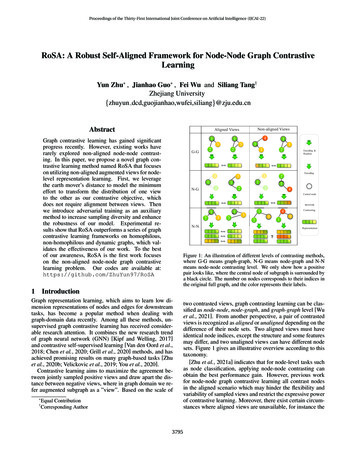
Proceedings of the Thirty-First International Joint Conference on Artificial Intelligence (IJCAI-22)large amount of information under a heterophilous setting andmakes the effort of other modules in vain.Thirdly and most importantly, RoSA outperforms otherbenchmarks on all three datasets, no matter the choice of theencoder, which validates the effectiveness of RoSA for heterophilous graphs. We speculate that RoSA will tighten thedistance of nodes of the same class.GraphSAGEGRACERoSAFlickrRedditRaw GMIGRACERoSA20.327.948.1 0.550.1 1.336.542.9 0.144.5 0.248.0 0.151.2 0.158.532.489.5 1.292.1 1.190.894.0 0.195.0 0.094.2 0.095.2 0.0Table 3: Result for inductive learning on large-scale datasets.Results for dynamic graphs dataset. In addition, we alsotest our method on dynamic graphs. For the contrastive task,we consider the adjacent snapshots as positive views becausethe evolution process is generally ”smooth”, and the snapshots far away from the anchor are considered as negativeviews. In CIAW, each snapshot maintains all nodes appearedin the timeline, however, in real-world scenarios, the additionor deletion of nodes happens as time goes by. So in CIAW*,we remove isolated nodes in each snapshot to emulate such asituation. Note that GRACE can not work on CIAW* becauseCIAW* creates a non-aligned situation, while GRACE is inherently an aligned method. From the statistics in Table 4,RoSA surpasses other competitors and can work well in bothsituations. Currently, we simply use static GNN encoder withdiscrete-time paradigms which can be replaced with temporalGNN encoders, and we will leave it for future work.4.4Ablation StudyTo prove the effectiveness of the design of RoSA, we conductablation experiments masking different components under the3800CIAW*64.0 8.565.3 7.967.6 7.069.7 10.173.2 9.3Table 4: Node classification using GraphSAGE on dynamic graphs.Result for inductive learning on large-scale datasets.The experiments conducted above are all under the transductive setting. In this part, the experiments are under the inductive setting where tests are conducted on unseen or untrainednodes. The micro-averaged F1 score is used for both of thesetwo datasets. The results are shown in Table 3, we can seethat RoSA works well on large-scale graphs under inductivesetting and reaches state-of-the-art performance. An explanation is DGI, GMI and GRACE can not directly work on fullgraphs, they use the sampling strategy proposed by [Hamilton et al., 2017] in their original work. However, we adoptsubsampling (random walk) as our augmentation techniquewhich means our method can seamlessly work on these largegraphs. Furthermore, our pretext task is designed for suchsubsampling which is more suitable for large graphs.MethodsCIAWFigure 3: Abalation study on RoSAsame hyperparameters. First we replace the EMD-based InfoNCE loss with a regular cosine similarity metric, represented as RoSA w/o EMD (In order to make it computableunder such situation, we restrict the same amount of nodes forcontrasted views). Second we use the vanilla cost matrix forEMD, named as RoSA w/o TD. Then we remove the adversarial training process, denoted as RoSA w/o AT. Finally, weadopt aligned views contrasting instead of the original nonaligned random walking, named as RoSA Aligned. For a faircomparison, we keep other hyperparameters and the trainingscheme same. The results is summarized in Figure 3. As wecan see, the performance degrades without either EMD, adversarial training or rectified cost matrix, which indicates theeffectiveness of the corresponding components. Furthermore,compared to aligned views, the model achieves comparableor even better results under the non-aligned condition, whichdemonstrates that our model, to a certain degree, solves thenon-aligned graph contrasting problem. The experiments ofsensitivity analysis are in Appendix D.5ConclusionIn this paper, we propose a robust self-aligned frameworkfor node-node graph contrastive learning, where we designand utilize the graph-based earth mover’s distance (g-EMD)as a similarity measure in the contrastive loss to avoid explicit alignment between contrasted views. Then we introduce unsupervised adversarial training into graph domain tofurther improve the robustness of the model. Extensive experiment results on homophilous, non-homophilous and dynamic graphs datasets demonstrate that our model can effectively be applied to non-aligned situations and outperformother competitors. Moreover, in this work we adopt simplerandom walk with restart as the subsampling technique, andRoSA may achieve better performance if equipped with morepowerful sampling methods in future work.
Proceedings of the Thirty-First International Joint Conference on Artificial Intelligence (IJCAI-22)AcknowledgmentsThis work has been supported in part by NationalKey Research and Development Program of China(2018AAA0101900), Zhejiang NSF (LR21F020004),Key Research and Development Program of ZhejiangProvince, China (No. 2021C01013), Chinese KnowledgeCenter of Engineering Science and Technology (CKCEST),Zhejiang University iFLYTEK Joint Research Center.References[Chen et al., 2020] Ting Chen, Simon Kornblith, Mohammad Norouzi, and Geoffrey E. Hinton. A simple framework for contrastive learning of visual representations. InProc. of ICML, 2020.[Cuturi, 2013] Marco Cuturi
in non-aligned node-node graph contrastive learning. Our main contributions are summarized as follows: We propose a robust self-aligned contrastive learning framework for node-node graph representation learning named RoSA. To the best of our knowledge, this is the rst work dedicated to solving non-aligned node-node graph contrastive .