Transcription
ITSM-R Reference ManualGeorge WeigtFebruary 11, 2018Contents1 Introduction1.1 Time series analysis in a1.2 White Noise Variance .1.3 ARMA Coefficients . . .1.4 ARIMA Models . . . . .1.5 Data Sets . . . . . . . .nutshell. . . . . . . . . . . . . . . . .2234552 Functions2.1 aacvf . . . .2.2 acvf . . . . .2.3 ar.inf . . . .2.4 arar . . . . .2.5 arma . . . . .2.6 autofit . . .2.7 burg . . . . .2.8 check . . . .2.9 forecast . .2.10 hannan . . . .2.11 hr . . . . . .2.12 ia . . . . . .2.13 ma.inf . . . .2.14 periodogram2.15 plota . . . .2.16 plotc . . . .2.17 plots . . . .2.18 Resid . . . .2.19 season . . . .2.20 sim . . . . . .2.21 smooth.exp .2.22 smooth.fft .2.23 smooth.ma . .2.24 smooth.rank2.25 specify . . .2.26 test . . . . .2.27 trend . . . .2.28 yw . . . . . 3435.1
1IntroductionITSM-R is an R package for analyzing and forecasting univariate time series data. The intendedaudience is students using the textbook Introduction to Time Series and Forecasting by Peter J.Brockwell and Richard A. Davis. The textbook includes a student version of the Windows-basedprogram ITSM 2000. The initials ITSM stand for Interactive Time Series Modeling. ITSM-R providesa subset of the functionality found in ITSM 2000.The following example shows ITSM-R at work forecasting a time series.library(itsmr)plotc(wine)M c("log","season",12,"trend",1)e Resid(wine,M)test(e)a arma(e,p 1,q 1)ee Load ITSM-RPlot the dataModel the dataObtain residualsCheck for stationarityModel the residualsObtain secondary residualsCheck for white noiseForecast future valuesNote the use of Resid with a capital R to compute residuals. ITSM-R uses Resid instead of resid toavoid a name conflict warning when the library is loaded.1.1Time series analysis in a nutshellIt turns out that you do most of the work. You have to analyze the data and determine a data modelM and ARMA model a that yield white noise for residuals.Time series data M a White noiseWhat the software does is invert M and a to transform zero into a forecast. (Recall that zero is thebest predictor of noise.)0 a 1 M 1 ForecastModel M should yield residuals that are a stationary time series. Basically this means that any trendin the data is eliminated. (Seasonality in the data can be removed by either M or a.) The testfunction is used to determine if the output of M is stationary. The following is the result of test(e)in the above 020304001020LagResidualsNormal Q-Q Plot-0.1Sample Quantiles40-0.3-0.1-0.3300.1 0.2Lag0.1 0.20020406080100120140-2Index-10Theoretical Quantiles212
Null hypothesis: Residuals are iid noise.TestDistribution StatisticLjung-Box QQ chisq(20)71.57McLeod-Li QQ chisq(20)12.07Turning points T(T-93.3)/5 N(0,1)93Diff signs S(S-70.5)/3.5 N(0,1)70Rank P(P-5005.5)/283.5 N(0,1)5136p-value0 *0.91380.94680.88480.6453As seen above, the ACF and PACF plots decay rapidly indicating stationarity. After M is determined,the residuals of M are modeled with an ARMA model a. In some circumstances the following tablecan be useful for choosing p and q from the plots of test(e).ACFDecaysZero for h qDecaysPACFZero for h pDecaysDecaysModelAR(p)MA(q)ARMA(p, q)The ARMA model a should yield residuals that resemble white noise. To check for white noise, thetest function is used a second time. The following is the result of test(ee) in the above 020304001020LagResidualsNormal Q-Q Plot40-0.3-0.10.1-0.1-0.3300.1LagSample l QuantilesNull hypothesis: Residuals are iid noise.TestDistribution StatisticLjung-Box QQ chisq(20)13.3McLeod-Li QQ chisq(20)16.96Turning points T(T-93.3)/5 N(0,1)93Diff signs S(S-70.5)/3.5 N(0,1)70Rank P(P-5005.5)/283.5 N(0,1)4999p-value0.86420.65560.94680.88480.9817The vertical lines in the ACF and PACF plots are below the noise threshold (the dashed horizontallines) for lags greater than zero which is good. In addition, the p-values in the table all fail to rejectthe null hypothesis of iid noise. Recall that a p-value is the probability that the null hypothesis is true.1.2White Noise VarianceITSM-R includes five methods for estimating ARMA parameters. They are Yule-Walker, Burg,Hannan-Rissanen, maximum likelihood, and the innovations method. For all estimation methods,ITSM-R uses the following formula to estimate white noise variance (Brockwell and Davis, p. 164).nσ̂ 2 1 X (Xt X̂t )2nrt 1t 13
The Xt X̂t are innovations (Brockwell and Davis, p. 71). Residuals are defined as follows (Brockwelland Davis, p. 164).Xt X̂tŴt rt 1Thus σ̂ 2 is the average of the squared residuals.The innovations algorithm (Brockwell and Davis, p. 73) is used to compute X̂t and rt 1 . Note that thealgorithm produces mean squared errors vt 1 E(Xt X̂t )2 for κ(i, j) E(Xi Xj ) given in equation(2.5.24). However, ITSM-R uses κ(i, j) E(Wi Wj ) given in equation (3.3.3). For the covariancein (3.3.3) the innovations algorithm produces rt 1 E(Wt Ŵt )2 instead of vt 1 . The relationshipbetween vt 1 and rt 1 is given in equation (3.3.8) asvt 1 E(Xt X̂t )2 σ 2 E(Wt Ŵt )2 σ 2 rt 1where σ 2 is white noise variance.It should be noted that γX in (3.3.3) is the autocovariance of the ARMA model, not of the data. Thenby equation (3.2.3) it can be seen that σ 2 in (3.3.3) cancels with σ 2 in γX . Hence the innovationsalgorithm does not depend on white noise variance at all. After the innovations are computed, whitenoise variance is estimated using the above formula for σ̂ 2 .γX (h) E(Xt h Xt ) σ 2 Xψj ψj h (3.2.3)j 0m max(p, q)κ(i, j) (3.3.2) 21 i, j m σ γ"X (i j), # p X σ 2 γX (i j) φr γX (r i j ) , min(i, j) m max(i, j) 2m, r 1q X θr θr i j , r 0 0(3.3.3)min(i, j) m,otherwise.Because all estimation methods use the above formula for σ̂ 2 , variance estimates computed by ITSM-Rare different from what is normally expected. For example, the Yule-Walker estimation function ywreturns a white noise variance estimate that differs from the traditional Yule-Walker algorithm.Since variance estimates are computed uniformly, model AICCs can always be compared directly, evenwhen different methods are used to estimate model parameters. For example, it is perfectly valid tocompare the AICC of a Yule-Walker model to that of a maximum likelihood model.1.3ARMA CoefficientsARMA coefficient vectors are ordered such that the vector index corresponds to the lag of the coefficient.For example, the modelXt φ1 Xt 1 φ2 Xt 2 Zt θ1 Zt 1 θ2 Zt 24
withφ1 1/2φ2 1/3θ1 1/4θ2 1/5corresponds to the following R vectors.phi c(1/2,1/3)theta c(1/4,1/5)The equivalent modelXt φ1 Xt 1 φ2 Xt 2 Zt θ1 Zt 1 θ2 Zt 2makes plain the sign convention of the AR coefficients.1.4ARIMA ModelsARIMA(p,d,q) models are specified by differencing d times with a lag of one each time. For example,the following R code specifies an ARIMA(1,2,3) model for data set quant.M c("diff",1,"diff",1)e Resid(quant,M)a arma(e,1,3)1.5Data SetsITSM-R includes the following data sets that are featured in Introduction to Time Series and Forecasting. Each data set is an ordinary vector (not a time series neObs.14472789830100142DescriptionNumber of international airline passengers, 1949 to 1960USA accidental deaths, 1973 to 1978Dow Jones utilities index, August 28 to December 18, 1972Level of Lake Huron, 1875 to 1972USA union strikes, 1951 to 1980Number of sunspots, 1770 to 1869Australian red wine sales, January 1980 to October 19915
22.1FunctionsaacvfComputes the autocovariance of an ARMA model. aacvf(a,h)a ARMA modelh Maximum lagThe ARMA model is a list with the following components. phi theta sigma2AR coefficients [1:p] φ1 , . . . , φpMA coefficients [1:q] θ1 , . . . , θqWhite noise variance σ 2Returns a vector of length h 1 to accomodate lag 0 at index 1.The following example is from p. 103 of Introduction to Time Series and Forecasting.R a specify(ar c(1,-0.24),ma c(0.4,0.2,0.1))R aacvf(a,3)[1] 7.171327 6.441393 5.060274 3.6143406
2.2acvfComputes the autocovariance of time series data. acvf(x,h 40)x Time series datah Maximum lagReturns a vector of length h 1 to accommodate lag 0 at index 1.Example:5000gamma1000R gamma acvf(Sunspots)R plot(0:40,gamma,type "h")010200:4073040
2.3ar.infReturns the AR( ) coefficients π0 , π1 , . . ., πn where π0 1. ar.inf(a,n)a ARMA modeln OrderA vector of length n 1 is returned to accommodate π0 at index 1.Example:R a yw(Sunspots,2)R ar.inf(a,10)[1] 1.0000000 -1.3175005[7] 0.0000000 00000.00000000.0000000For invertible ARMA processes, AR( ) is the polynomial π(z) such thatπ(z) φ(z) 1 π1 z π2 z 2 · · ·θ(z)The corresponding autoregression isZt π(B)Xt Xt π1 Xt 1 π2 Xt 2 · · ·The coefficients πj are calculated recursively using the following formula. (See p. 86 of Introduction toTime Series and Forecasting.)πj φj qXθk πj kk 18j 1, 2, . . .
2.4ararPredict future values of a time series using the ARAR algorithm.arar(x,h 10,opt 2) Observed data xhSteps ahead opt Display optionThe display options are 0 for silent, 1 for tabulate, 2 for plot and tabulate. Returns the following listinvisibly. pred se l uPredicted valuesStandard errorsLower boundsUpper boundsExample:100200300400500600700R arar(airpass)Optimal lags 1 2 9 10Optimal coeffs 0.5247184 0.2735903 0.2129203 -0.316453WN Variance 110.1074Filter 1 -0.5247184 -0.2735903 0 0 0 0 0 0 -0.2129203 0.316453 0-1.114253 0.5846688 0.3048487 0 0 0 0 0 0 0.237247 -0.3526086StepPredictionsqrt(MSE)Lower BoundUpper 10518.513515.93834487.2743549.75260501009150
2.5armaReturns an ARMA model using maximum likelihood to estimate the AR and MA coefficients.arma(x,p 0,q 0) x Time series datap AR order q MA orderThe R function arima is called to estimate φ and θ. The innovations algorithm is used to estimate thewhite noise variance σ 2 . The resulting ARMA model is a list with the following components. phi theta sigma2 aicc se.phi se.thetaAR coefficients [1:p] φ1 , . . . , φpMA coefficients [1:q] θ1 , . . . , θqWhite noise variance σ 2Akaike information criterion correctedStandard errors for the AR coefficientsStandard errors for the MA coefficientsThe signs of the coefficients correspond to the following model.Xt pXφj Xt j Zt j 1qXθk Zt kk 1The following example estimates ARMA(1,0) parameters for a stationary transformation of the DowJones data.R M c("diff",1)R e Resid(dowj,M)R a arma(e,1,0)R a phi[1] 0.4478187 theta[1] 0 sigma2[1] 0.1455080 aicc[1] 74.48316 se.phi[1] 0.01105692 se.theta[1] 010
2.6autofitUses maximum likelihood to determine the best ARMA model given a range of models. The autofitfunction tries all combinations of argument sequences and returns the model with the lowest AICC.This is a wrapper function, the R function arima does the actual estimation.autofit(x,p 0:5,q 0:5) x Time series datap AR order q MA orderReturns a list with the following components. phi theta sigma2 aicc se.phi se.thetaAR coefficients [1:p] φ1 , . . . , φpMA coefficients [1:q] θ1 , . . . , θqWhite noise variance σ 2Akaike information criterion correctedStandard errors for the AR coefficientsStandard errors for the MA coefficientsThe signs of the coefficients correspond to the following model.Xt pXφj Xt j Zt j 1qXθk Zt kk 1The following example shows that an ARMA(1,1) model has the lowest AICC for the Lake Huron data.R autofit(lake) phi[1] 0.7448993 theta[1] 0.3205891 sigma2[1] 0.4750447 aicc[1] 212.7675 se.phi[1] 0.006029624 se.theta[1] 0.0128889411
2.7burgEstimates AR coefficients using the Burg method. burg(x,p)x Time series datap AR orderReturns an ARMA model with the following components. phi theta sigma2 aicc se.phi se.thetaAR coefficients [1:p] φ1 , . . . , φp0White noise variance σ 2Akaike information criterion correctedStandard errors for AR coefficients0Example:R burg(lake,1) phi[1] 0.8388953 theta[1] 0 sigma2[1] 0.5096105 aicc[1] 217.3922 se.phi[1] 0.003023007 se.theta[1] 012
2.8checkCheck for causality and invertibility of an ARMA model.check(a) a ARMA modelThe ARMA model is a list with the following components. phi thetaAR coefficients [1:p] φ1 , . . . , φpMA coefficients [1:q] θ1 , . . . , θqExample:R a specify(ar c(0,0,0.99))R check(a)CausalInvertible13
2.9forecastPredict future values of a time series.forecast(x,M,a,h 10,opt 2,alpha 0.05) x M ah opt alphaTime series dataData modelARMA modelSteps aheadDisplay optionLevel of significanceThe data model M can be NULL for none. The display options are 0 for none, 1 for tabulate, 2 for plotand tabulate. See below for details about the data model.Example:Upper 2500300035004000R M c("log","season",12,"trend",1)R e Resid(wine,M)R a arma(e,1,1)R forecast(wine,M,a)StepPredictionLower 510.185103180.4182577.324050100150The data model M is a vector of function names. The functions are applied to the data in left to rightorder. There are five functions from which to choose.14
diffhrlogseasontrendDifference the dataSubtract harmonic componentsTake the log of the dataSubtract seasonal componentSubtract trend componentA function name may be followed by one or more arguments.diff has a single argument, the lag.hr has one or more arguments, each specifying the number of observations per harmonic period.log has no arguments.season has one argument, the number of observations per season.trend has one argument, the polynomial order of the trend, (1 for linear, 2 for quadratic, etc.)A data model is built up by concatenating the function names and arguments. For example, thefollowing vector takes the log of the data, then subtracts a seasonal component of period twelve thensubtracts a linear trend component.R M c("log","season",12,"trend",1)At the end of the data model there is an implied subtraction of the mean operation. Hence the resultingtime series always has zero mean.15
2.10hannanEstimates ARMA coefficients using the Hannan-Rissanen algorithm. It is required that q 0.hannan(x,p,q) x Time series datap AR order q MA orderReturns a list with the following components. phi theta sigma2 aicc se.phi se.thetaAR coefficients [1:p] φ1 , . . . , φpMA coefficients [1:q] θ1 , . . . , θqWhite noise variance σ 2Akaike information criterion correctedStandard errors for AR coefficientsStandard errors for MA coefficientsExample:R hannan(lake,1,1) phi[1] 0.6960772 theta[1] 0.3787969 sigma2[1] 0.477358 aicc[1] 213.183 se.phi[1] 0.07800321 se.theta[1] 0.146526516
2.11hrReturns the sum of harmonic components of time series data. hr(x,d)x Time series datad Vector of harmonic periodsExample:7000800090001000011000R y hr(deaths,c(12,6))R plotc(deaths,y)01020304017506070
2.12iaCalculates MA coefficients using the innovations algorithm.ia(x,q,m 17) x Time series dataq MA order m Recursion levelReturns a list with the following components. phi theta sigma2 aicc se.phi se.theta0MA coefficients [1:q] θ1 , . . . , θqWhite noise variance σ 2Akaike information criterion corrected0Standard errors for MA coefficientsNormally m should be set to the default 17 even when fewer MA coefficients are required.The following example generates results that match Introduction to Time Series and Forecasting p.154.R y diff(dowj)R a ia(y,17)R round(a theta,4)[1] 0.4269 0.2704 0.1183 0.1589[9] 0.0148 -0.0017 0.1974 -0.0463[17] 0.0760R round(a theta/a se/1.96,4)[1] 1.9114 1.1133 0.4727 0.6314[9] 0.0568 -0.0064 0.7594 -0.1757[17] 0.27600.13550.20230.1568 0.1284 -0.00600.1285 -0.0213 -0.25750.53310.76660.6127 0.4969 -0.02310.4801 -0.0792 -0.9563The formula for the standard error of the jth coefficient is given on p. 152 of Introduction to TimeSeries and Forecasting as" j 1#1/2X2σj n 1/2θ̂mii 0where θ̂m0 1. Hence the standard error for θ̂1 is σ1 n 1/2 .18
2.13ma.infReturns the MA( ) coefficients ψ0 , ψ1 , . . ., ψn where ψ0 1. ma.inf(m,n)a ARMA modeln OrderA vector of length n 1 is returned to accommodate ψ0 at index 1.Example:R a yw(Sunspots,2)R ma.inf(a,10)[1] 1.00000000 1.31750053 1.10168617 0.61601672 0.11299949[6] -0.24175256 -0.39016452 -0.36074148 -0.22786538 -0.07145884[11] 0.05034727For causal ARMA processes, MA( ) is the polynomial ψ(z) such thatψ(z) θ(z) 1 ψ1 z ψ2 z 2 · · ·φ(z)The corresponding moving average isXt ψ(B)Zt Zt ψ1 Zt 1 ψ2 Zt 2 · · ·The coefficients ψj are calculated recursively using the following formula. (See p. 85 of Introductionto Time Series and Forecasting.)ψj θj pXφk ψj kk 119j 1, 2, . . .
2.14periodogramPlots a periodogram. Time series data xqMA filter order opt Plot optionperiodogram(x,q 0,opt 2)The periodogram vector divided by 2π is returned invisibly. The plot options are 0 for no plot, 1 toplot only the periodogram, and 2 to plot both the periodogram and the filter coefficients. The filterq can be a vector in which case the overall filter is the composition of MA filters of the designatedorders.R periodogram(Sunspots,c(1,1,1,1))Filter 0.01234568 0.04938272 0.1234568 0.1975309 0.2345679 0.1975309 0.12345680.04938272 0.012345680400800(Smoothed hing Filter246208
2.15plotaPlots ACF and PACF for time series data and/or ARMA model. plota(u,v NULL,h 40)u, v Time series data and/or ARMA model, in either orderhMaximum lagExample:R -0.50.00.5Data010203040010Lag203040LagR a yw(Sunspots,2)R 1.0-1.0-0.50.00.5DataModel0102030400Lag10203040Lag The following example demonstrates the utility of the 1.96/ n bounds as a test for noise.R noise rnorm(200)R plota(noise)21
102030400Lag1020Lag223040
2.16plotcPlots one or two time series in color. plotc(y1,y2 NULL)y1 Blue line with knotsy2 Red line without knotsExample:050100150200R 150200R y trend(uspop,2)R plotc(uspop,y)23
2.17plotsPlots the spectrum of data or an ARMA model.plots(u) u Time series data or ARMA modelExample:R a specify(ar c(0,0,0.99))R plots(a)Model Spectrum0.00.51.01.5242.02.53.0
2.18ResidReturns the residuals of a time series model.Resid(x,M NULL,a NULL) x Time series dataM Data model a ARMA modelEither M or a can be NULL for none. See below for details about the data model. The returned residualsalways have zero mean.In the following example, Resid and test are used to check for stationarity of the transformed data.Then they are used again to check that the overall model reduces the data to white noise.R R R R R R M c("log","season",12,"trend",1)e Resid(airpass,M)test(e)a arma(e,1,0)ee Resid(airpass,M,a)test(ee)The data model M is a vector of function names. The functions are applied to the data in left to rightorder. There are five functions from which to choose.diffhrlogseasontrendDifference the dataSubtract harmonic componentsTake the log of the dataSubtract seasonal componentSubtract trend componentA function name may be followed by one or more arguments.diff has a single argument, the lag.hr has one or more arguments, each specifying the number of observations per harmonic period.log has no arguments.season has one argument, the number of observations per season.trend has one argument, the polynomial order of the trend, (1 for linear, 2 for quadratic, etc.)A data model is built up by concatenating the function names and arguments. For example, thefollowing vector takes the log of the data, then subtracts a seasonal component of period twelve thensubtracts a linear trend component. M c("log","season",12,"trend",1)At the end of the data model there is an implied subtraction of the mean operation. Hence the resultingtime series always has zero mean.25
2.19seasonReturns the seasonal component of time series data. season(x,d)x Time series datad Number of observations per seasonExample:-20000200040006000800010000R s season(deaths,12)R plotc(deaths,s)01020304026506070
2.20simGenerate synthetic observations for an ARMA model. sim(a,n)a ARMA modeln Number of synthetic observations requiredThe ARMA model is a list with the following components. phi theta sigma2AR coefficients φ1 , . . . , φpMA coefficients θ1 , . . . , θqWhite noise variance σ 2Example:-10-50510R a specify(ar c(0,0,0.99))R x sim(a,60)R plotc(x)010203027405060
2.21smooth.expApplies an exponential smoothing filter to data and returns the result. smooth.exp(x,a)x Time series dataa 0 to 1, zero is maximum smoothness.Example:350040004500500055006000R y smooth.exp(strikes,0.4)R plotc(strikes,y)05101528202530
2.22smooth.fftApplies a low pass filter to data and returns the result. smooth.fft(x,c)x Time series datac Cut-off freq. 0–1The cut-off frequency is specified as a fraction. For example, c 0.25 passes the lowest 25% of thefrequency spectrum.Example:-2-10123R y smooth.fft(signal,0.035)R plotc(signal,y)05010029150200
2.23smooth.maApplies a moving average filter to data and returns the result. smooth.ma(x,q)x Time series dataq Filter orderExample:350040004500500055006000R y smooth.ma(strikes,2)R plotc(strikes,y)0510152025From p. 25 of Introduction to Time Series and Forecasting,Yt qX1Xt j2q 1j qHence for q 2 the moving average filter is1Yt (Xt 2 Xt 1 Xt Xt 1 Xt 2 )53030
2.24smooth.rankPasses the mean and the k frequencies with the highest amplitude. The remainder of the spectrum isfiltered out. smooth.rank(x,k)x Time series datak RankExample:7000800090001000011000R y smooth.rank(deaths,1)R 090001000011000R y smooth.rank(deaths,2)R plot(deaths,y)031
2.25specifyReturns an ARMA model with the specified parameters.specify(ar 0,ma 0,sigma2 1) AR coefficients [1:p] φ1 , . . . , φp armaMA coefficients [1:q] θ1 , . . . , θq sigma2 White noise variance σ 2The signs of the coefficients correspond to the following model.Xt φ1 Xt 1 φ2 Xt 2 · · · Zt θ1 Zt 1 θ2 Zt 2 · · ·Example:R specify(ar c(0,0,0.99)) phi[1] 0.00 0.00 0.99 theta[1] 0 sigma2[1] 132
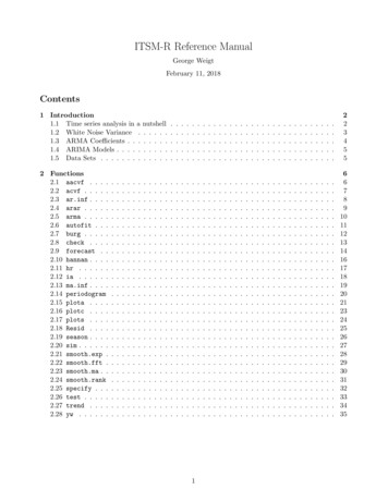
2.26testTest residuals for randomness.test(e) e ResidualsExample:R M c("log","season",12,"trend",1)R e Resid(airpass,M)R test(e)Null hypothesis: Residuals are iid noise.TestDistribution StatisticLjung-Box QQ chisq(20)412.43McLeod-Li QQ chisq(20)41.29Turning points T(T-94.7)/5 N(0,1)85Diff signs S(S-71.5)/3.5 N(0,1)68Rank P(P-5148)/289.5 N(0,1)5187p-value0 *0.0034 1.0-0.50.00.5Data1020304001020LagResidualsNormal Q-Q Plot40-0.15-0.050.05-0.05-0.15300.05LagSample Quantiles0020406080100120140-2Index-10Theoretical Quantiles3312
2.27trendReturns the trend component of time series data. trend(x,p)x Time series datan Polynomial orderExample:050100150200250R y trend(uspop,2)R plotc(uspop,y)180018501900341950
2.28ywEstimates AR coefficients using the Yule-Walker method. yw(x,p)x Time series datap AR orderReturns an ARMA model with the following components. phi theta sigma2 aicc se.phi se.thetaAR coefficients [1:p] φ1 , . . . , φp0White noise variance σ 2Akaike information criterion correctedStandard errors for AR coefficients0Example:R yw(lake,1) phi[1] 0.8319112 theta[1] 0 sigma2[1] 0.5098608 aicc[1] 217.4017 se.phi[1] 0.003207539 se.theta[1] 0These are the relevant formulas from Introduction to Time Series and Forecasting, Second Edition.n h 1 Xγ̂(h) Xt h X̄n Xt X̄nn(2.4.4)t 1 · · · γ̂(k 1) · · · γ̂(k 2) Γ̂k . .γ̂(k 1) γ̂(k 2) · · ·γ̂(0)γ̂(0)γ̂(1).γ̂(1)γ̂(0).R̂k 1Γ̂kγ̂(0)35(2.4.6)(2.4.8)
φ̂p R̂p 1 ρ̂p(5.1.7) v̂p γ̂(0) 1 ρ̂0p R̂p 1 ρ̂p(5.1.11)where ρ̂p (ρ̂(1), . . . , ρ̂(p))0 γ̂p /γ̂(0). The subscript p is the order of the AR model (i.e., number ofAR coefficients). Note that (5.1.7) and (5.1.11) can also be written asφ̂p Γ̂ 1p γ̂pandv̂p γ̂(0) γ̂p0 φ̂pFrom equation (5.1.13) the standard error for the jth AR coefficient isrv̂jjSEj nwhere v̂jj is the jth diagonal element of v̂p Γ̂ 1p .The R code follows immediately from the above equations.gamma acvf(x,p)Gamma toeplitz(gamma[1:p])phi solve(Gamma,gamma[2:(p 1)])v gamma[1] - drop(crossprod(gamma[2:(p 1)],phi))V v * solve(Gamma)se.phi sqrt(1/n*diag(V))Recall that R indices are 1-based hence gamma[1] is γ̂(0). The function crossprod returns a 1-by-1matrix which is then converted by drop to a scalar.36
ITSM-R is an R package for analyzing and forecasting univariate time series data. The intended audience is students using the textbook Introduction to Time Series and Forecasting by Peter J. Brockwell and Richard A. Davis. The textbook includes a student version of the Windows-based program ITSM 2000.