WIXLIB

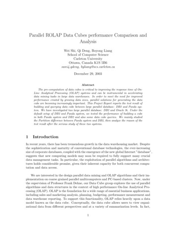
3.2Query3.2.1Build Multiple Index - RcubeParallel RCUBE Index Generator - rcube.exe The RCUBE index generation module buildsmulti-dimensional packed r-tree indexes for the data cube constructed by the data cubegenerator. Specifically, it will build a separate index for each of the O(2d) aggregate viewsthat have been previously distributed across the cluster[5].With respect to the output, a pair of files will actually be generated for each data cubeview. The first is a Hilbert-sorted data set. Simply put, this file is a reorganization of theaggregate view in Hilbert order. Moreover, the records are organized into block sized units.Records do not cross block boundaries and padding is used where necessary[5].The second file is the index proper. It is a tree-based construct that provides access tothe records contained in the blocks of the Hilbert sorted data set[5].Unlike the original data cube, the index files are not localized on a given disk. Instead,each Hilbert/Index pair is striped across every disk. Each Hilbert/Index pair represents apartial index that will, in turn, be used by the query generator[5].3.2.2Parallel Query EngineThe query engine module accepts multi-dimensional user queries and resolves them againstthe indexed data cube produced by the data cube and index generators. Queries can eitherbe point queries, range queries or, in special cases, hierarchical queries[5].44.1DB2 Parallel ComputingArchitecturep1 - share nothingDB2 PE employs a Shared noting architecture in which the database system consists of a setof independent logical database nodes. Each logical node represents a collection of systemresources including, processes, main memory, disk storage and communications, managedby an independent database manager. The logical nodes use message passing to exchangedata with each other. Tables are partitioned across nodes using a hash partitioning strategy.The cost-based parallel query optimizer takes table partitioning information into accountwhen generating parallel plans for execution by the runtime system. A DB2 PE system canbe configured to contain one or more logical nodes per physical processor. For example,the system can be configured to implement one node per processor in a shared-nothing,MPP system or multiple nodes in a symmetric multiprocessor (SMP) system. This paperprovides an overview of the storage model, query optimization, runtime system, utilities,and performance of DB2 Parallel Edition. See figure 2p2 - share nothingDB2 PE supports a partitioned storage model I which tables in a database are partitioned5

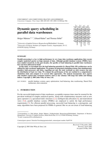
Figure 2: DB2 parallel computing architectureacross a set of database nodes. Indexes are partitioned along with their corresponding talesand stored locally at each node. The system supports hash partitioning and partial declustering a of database tables. Extensions to the CREATE TABLE statement allow users tospecify a partitioning key and nodegroup associated with a table. The partitioning keyis a set of columns in the table row is stored. Nodegroups are named subsets of databasenodes. Each nodegroup is associated with a data structure called the partitioning map(PM)partitioning map (PM) which consists of 4096 entries each containing a node number. Ifx represents the partitioning key value of a row in a table, then node at which this row isstored is given by, PM (H) which consists of 4096 entries. If x represents the partitioningkey value of a row in a table, then the node at which this row is stored is given by, PM[H(x)],where H(.) represents the system hash function and PM represents the partitioning map associated with the nodegroup in which the table is created. Data definition language (DDL)extensions are provided to allow users to create nodegroups in a data base.4.2Partition mechanismDB2 Parallel Edition supports the hash partitioning technique to assign each row of a tableto the node to which the row is hashed. You need to define a partitioning key before applying the hashing algorithm. The hashing algorithm uses the partitioning key as an inputto generate a partition number. The partition number then is used as an index into thepartitioning map. The partitioning map contains the node number(s) of the nodegroup.There are three major steps to perform the data partitioning:6

Figure 3: Parallel DB2 Partition diagram1. Partitioning key selection: A partitioning key is a set of one or more columns of a giventable. It is used by the hashing algorithm to determine on which node the row is placed.2. Partitioning map creation: In DB2 Parallel Edition, a partitioning map is an array of4096 node numbers. Each nodegroup has a partitioning map. The content of the partitioning map consists of the node numbers which are defined for that nodegroup. The hashingalgorithm uses the partitioning key on input to generate a partition number. The partitionnumber has a value between 0 and 4095. It is then used as an index into the partitioningmap for the nodegroup. The node number in the partitioning map is used to indicate towhich node the operation should be sent.3. Partitioning rows: The steps for row partitioning consist of splitting and inserting thedata across the target nodes. DB2 Parallel Edition provides tools to partition the data andthen load the data to the system via a fast-load utility or import. Data can also be insertedinto the database via an application that uses buffered inserts. See figure 34.3Table - Table Space - Partition RoupNodegroups and Data PartitioningIn DB2 Parallel Edition, data placement is one of the more challenging tasks. It determinesthe best placement strategy for all tables defined in a parallel database system. The rows ofa table can be distributed across all the nodes (fully declustered), or a subset of the nodes(partially declustered). Tables can be assigned to a particular set of nodes. Two tables in aparallel database system can share exactly the same set of nodes (fully overlapped), at leastone node (partially overlapped), or no common nodes (nonoverlapped). Parallel Editionsupports the hash partitioning technique to assign a row of a table to a table partition.Nodegroups7

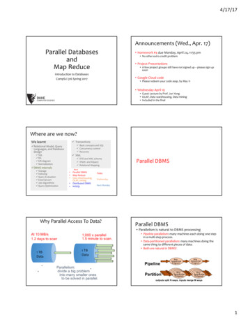
Figure 4: Nodegroup diagramNodegroups in DB2 Parallel Edition are used to support declustering (full or partial), overlapped assignment and hash partitioning of tables in the parallel database system. Anodegroup is a named subset of one or more of the nodes defined in the node configuration file, HOME/sqllib/db2nodes.cfg, of DB2 Parallel Edition. It is used to managethe distribution of table partitions. In DB2 Parallel Edition, there are system-defined anduser-defined nodegroups. Tables must be created within a nodegroup. Figure xx shows aDB2 Parallel Edition instance consisting of four physical machines. The default nodegroup,IBMDEFAULTGROUP, spans all of the nodes in the instance. The catalog nodegroup,IBMCATGROUP, is created only on the node where the create database command wasissued. The catalog node is on host0 in this example. Also shown is a user-defined groupthat spans host2 and host3. See figure 4.4.4Query optimize and summary table MQTWe use CUBE grouping to generate full data cube in DB2. CUBE grouping is an extensionto the GROUP BY clause that produces a result set that contains all the rows of a ROLLUPaggregation. A CUBE grouping can also be thought of as a series of grouping-sets. In thecase of a CUBE, all permutations of the cubed grouping-expression-list are computed alongwith the grand total. Therefore, the n elements of a CUBE translate to 2**n (2 to thepower n) grouping-sets[1]. The following is an example of create full data cube using CUBEgrouping:8

SELECT a, b, c, d, e, f, sum(fact) as amount,COUNT(fact) AS COUNTAMOUNT FROM fact8GROUP BY CUBE (a, b, c, d, e, f)We use materialized query table (MQT) that stores the results of CUBE grouping to issuethe cube query. DB2 optimizer will automatically choose MQT if a range query happenson the base table.The following is an example of create full data cube as MQT.CREATE TABLE fact8cubeAS (SELECT a, b, c, d, e, f, sum(fact) as amount, COUNT(fact) AS COUNT AMOUNTFROM fact8GROUP BY CUBE (a, b, c, d, e, f))DATA INITIALLY DEFERRED REFRESH IMMEDIATEENABLE QUERY OPTIMIZATIONIN cubets8The REFRESH TABLE statement refreshes the data in a MQT, in our case, builds the fulldata cube.5Experiment EvaluationIn this section, we present and compare experimental results for the parallel full cube generation and parallel cube query in Panda system and DB2 Parallel Edition V8.0 system.We will also discuss the experimental DB2 environment that might infect the system performance.We use Panda’s Data Generator to generate a group of data which contains difference number of records, dimensions and cardinalities. The data are used to build full data cube andquery on 1 to 11 processors in Panda system. The same data are loaded into DB2 tablesand are used to build full data cube and query on 1 to 11 processors in DB2 system as well.We use the default configuration on both systems and ignore the CPU workload, systembuffer and others factors which might affect the performance.5.1Full data cube generationWe use Panda’s data cube generator utility in Panda system (see section 3.1). In DB2system, we use Materialized Query Tables (MQT) for cube groupBy (see section 4.3).We noticed that in Figure 5.2, the run time of building data cube on 8 nodes in DB2is extremely fast. It occurred when rebuild the cube several times, the buffer system insidethe DBMS might accelerate the performance.5.2Parallel Cube QueryWe use Panda’s parallel indexes generator and query engine utilities for data cube query inPanda system (see section 3.2, 3.3). We use MQT optimization mechanism for cube queryin DB2Figure 5is the run time of four parallel query run time of 1M data on Panda and DB29

Figure 5: Parallel query run time of 1M data on Panda and DB2 system (file query36.xsl)Figure 6: The run time of four parallel query on 8 processor for 1M and 2M data on Pandaand DB2 system(file query63.xsl)system. Figure6 is the run time of four parallel query on 8 processor for 1M and 2M dataon Panda and DB2 system.6Analysis and conclusionNOTE: Because there are only two groups of experimental result, the following analyzeand conclusion are based on the current result and to be proved and confirmed by moreexperimental.6.1Parallel data cube generationFigure 7 and 8 show that the run time of Panda’s parallel full data cube generation is muchfaster than DB2 system. The result also shows Panda system can balance the workload verywell, if we consider the average run-time of generation, Panda’s algorithm has very stablespeedup in most cases. DB2 system also has good speedup, but the result of partial data10

Figure 7: Test Result 1Figure 8: Test Result 2cube generation (groupBy MQT result in experimental report) shows in many case, the runtime might increase depends on data volume and partition number, say 11 partitions6.2Parallel data cube queryFigure 5 and 6 show that the run time of Panda’s parallel data cube query is extremelyfaster than DB2Of course, we realized that Panda has to take long to build multiple dimension indexesbefore it can handle queries. Consider we are working on the data warehouse, taking timeto build efficient index is worth to prompt the performance of the coming huge number ofqueries. We also realized we do not take the benefit of DB2 index mechanism to achievethe highest performance of DB2 query.11

6.3The efficient of data cube organizationThe experimental result shows Panda’s data cube and indexes partition is very efficient forcube query We realized that, unlike Panda system, DB2 PE, as a commercial DBMS, isdesigned to handle large number of concurrent transactions processing. Its high availability and reliability features, such as Logging system, Lock mechanism, will counteract thesystem to achieve highest performance.7Future WorkDue to the restriction of current experimental DB2 environment, our next work is to reviewthe comparisons of parallel data cube generation and query on more processors and largerdata volume. Analyze the performance for various kind of data cube, including the differentdimension numbers and cardinalities To reach the high performance of OLAP operation inDB2 system, we will also keep on researching DB2 data organization and partition mechanism. DB2 OLAP facilities, such as Cube View, OLAP Server, are also the interestingrelative topics we will work on.88.1AppendixExperiment ReportTargetAnalyze the data partition mechanism in RDBMSImplementing the data cube functionalities in parallel DB2 systemsRunning the Panda system and DB2 parallel data cube building and query to compare andanalyze the performance of these to systemSteps a) Data generate and transform Data generator -fHex Transform to text file -fTxtb) Panda Run the Panda cube building (pipesort.exe) and cube query(query.exe) based thedata file -fHex See previous filesc) DB2 Run the DB2 parallel cube building (refresh MQT) and cube query(summary table)based the data file -fHexi. DB2 environment setupDefine database - testcubeAdjust transaction logsDefine the partition group ’datacubegroup x’, where x means the number of nodes (1, 2, 4,8,13) Define the tabespaces on deferent nodes as following: ’cubets x’, where x means thenumber of nodes(1,2, 4, 8,13), in the corresponding ’datacubegroup x’already defined, just use them in the coming stepsii. Create base tablesCreate the base table in the corresponding tablesspaceNaming convention: factXdYp X: number of dimensions of data OR the sequence numberof testing Y: number of partition On the tablespace - ”cubetsY”Statement: db2 ”create table fact6d8p ( a int not null, b int not null, c int not null, d intnot null, e int not null, f int not null, fact int) IN cubets8 index in cubets8”12

iii. Load data to base tablecopy data file (in text format) into current node, say c1-2 scp input.dat oad dataiv. Define cube and buildDefine the cube(MQT) on the same tablespace as its base table FactXdYpCube On thesame tablespace- ”cubetsY” for the base table ”factXdYp”Stepsa) Define cubes: db2batch -d testcube -f build.sql -r build.resultb) Build (refresh) db2batch -d testcube -f rAll -r rAll.resultc) Check test result in rAll.resultv. Cube queryQuery”db2batch -d testcube -f mqt ex.sql -r mqt.result”Explaindb2expln -d testcube -f mqt ex.sql -o tempResult mqt.result2. result see the result file, collect data into the table and analyze.8.1.1Data combination1. Data size123500k 1M 2M2. Number of dimensions1236 8 103.Shew1230124. Cadinalities123high mix lowhigh: 256,256,256,256,.mix: 256,128,64,32,16,8,6,6,.low: 16,16,16,16,16,16,16,16,.5. Processors: 2,4,6,8,13Add a check mark at at the end of the data you’ve tested,1) 500k, 6, 0, high x13

,500k,6,6,6,6,6,6,6,6,0, mix0, low1, high1, mix1, low2,high2,mix2,low11)12)13)14)15)16)17)18)10) 500k, 8, 0, high500k, 8, 0, mix500k, 8, 0, low500k, 8, 1, high500k, 8, 1, mix500k, 8, 1, low500k, 8, 2,high500k, 8, 2,mix500k, 8, 2,low20)21)22)23)24)25)26)27)19) 500k, 10, 0, high500k, 10, 0, mix500k, 10, 0, low500k, 10, 1, high500k, 10, 1, mix500k, 10, 1, low500k, 10, 2,high500k, 10, 2,mix500k, 10, 2,low29)30)31)32)33)34)35)36)28) 1M, 6, 0, high1M, 6, 0, mix1M, 6, 0, low1M, 6, 1, high1M, 6, 1, mix1M, 6, 1, low1M, 6, 2,high1M, 6, 2,mix1M, 6, 2,low38)39)40)41)42)43)44)45)37) 1M, 8, 0, high1M, 8, 0, mix1M, 8, 0, low1M, 8, 1, high1M, 8, 1, mix1M, 8, 1, low1M, 8, 2,high1M, 8, 2,mix1M, 8, 2,low14

47)48)49)50)51)52)53)54)46) 1M, 10, 0, high1M, 10, 0, mix1M, 10, 0, low1M, 10, 1, high1M, 10, 1, mix1M, 10, 1, low1M, 10, 2, high1M, 10, 2, mix1M, 10, 2, low56)57)58)59)60)61)62)63)55) 2M, 6, 0, high2M, 6, 0, mix2M, 6, 0, low2M, 6, 1, high2M, 6, 1, mix2M, 6, 1, low2M, 6, 2,high2M, 6, 2,mix2M, 6, 2,low65)66)67)68)69)70)71)72)64) 2M, 8, 0, high2M, 8, 0, mix2M, 8, 0, low2M, 8, 1, high2M, 8, 1, mix2M, 8, 1, low2M, 8, 2,high2M, 8, 2,mix2M, 8, 2,low73) 2M, 10, 0, high74) 2M, 10, 0, mix75) 2M, 10, 0, low76) 2M, 10, 1, high77) 2M, 10, 1, mix78) 2M, 10, 1, low79) 2M, 10, 2,high80) 2M, 10, 2,mix81) 2M, 10, 2,lowReferences[1] Ibm db2 universal database sql reference version 8.15

[2] F. Carino and W. Sterling. Parallel strategies and new concepts for a petabyte multimedia database computer,. Parallel Database Techniques, M. Abdelguerfi and K.F.Wong, eds., chapter 7, IEEE CS Press, Los Alamitos, CA, pages pp. 139–164, 1998.[3] F. Dehne, T. Eavis, S. Hambrusch, and A. Rau-Chaplin. Parallelizing the data cube.Distributed and Parallel Databases, 11(2):181–201, 2002.[4] F. Dehne, T. Eavis, and Andrew Rau-Chaplin. A cluster architecture for parallel datawarehousing. In Proc IEEE International Conference on Cluster Computing and theGrid (CCGrid 2001), Brisbane, Australia, 2001.[5] T. Eavis. Parallel relational olap. June, 2003.[6] S. Goil and A. Choudhary. High performance OLAP and data mining on parallelcomputers. Journal of Data Mining and Knowledge Discovery, 1(4):391–417, 1997.[7] S. Goil and A. Choudhary. A parallel scalable infrastructure for OLAP and data mining.In Proc. International Data Engineering and Applications Symposium (IDEAS’99),Montreal, 1999.[8] David J. DeWitt J. Gray. Parallel database systems: The future of high performancedatabase processing,. January 1992.[9] H. Lu, X. Huang, and Z. Li. Computing data cubes using massively parallel processors.In Proc. 7th Parallel Computing Workshop (PCW’97), Canberra, Australia, 1997.[10] Seigo Muto and Masaru Kitsuregawa. A dynamic load balancing strategy for paralleldatacube computation. In ACM Second International Workshop on Data Warehousingand OLAP (DOLAP 1999), pages 67–72, 1999.[11] R.T. Ng, A. Wagner, and Y. Yin. Iceberg-cube computation with pc clusters. In ACMSIGMOD Conference on Management of Data, pages 25–36, 2001.16

the data cube model is central to our parallelization efforts[5]. Usually the size of the data cube is potentially very large. In order to meet the need for improved performance created by growing data sizes in OLAP applications, parallel solu-tions for generating the data cube have become increasingly important. The current parallel