Transcription
IEEE TRANSACTIONS ON BIOMEDICAL ENGINEERING, VOL. 68, NO. 1, JANUARY 2021247Machine-Learning Based Model to ImproveInsulin Bolus Calculation in Type 1Diabetes TherapyGiulia Noaro , Student Member, IEEE, Giacomo Cappon , Martina Vettoretti , Giovanni Sparacino ,Simone Del Favero , and Andrea FacchinettiAbstract—Objective: This paper aims at proposing anew machine-learning based model to improve the calculation of mealtime insulin boluses (MIB) in type 1 diabetes(T1D) therapy using continuous glucose monitoring (CGM)data. Indeed, MIB is still often computed through the standard formula (SF), which does not account for glucoserate-of-change (ΔG), causing critical hypo/hyperglycemicepisodes. Methods: Four candidate models for MIB calculation, based on multiple linear regression (MLR) and leastabsolute shrinkage and selection operator (LASSO) are developed. The proposed models are assessed in silico, usingthe UVa/Padova T1D simulator, in different mealtime scenarios and compared to the SF and three ΔG-accountingvariants proposed in the literature. An assessment on realdata, by retrospectively analyzing 218 glycemic traces, isalso performed. Results: All four tested models performedbetter than the existing techniques. LASSO regression withextended feature-set including quadratic terms (LASSOQ )produced the best results. In silico, LASSOQ reduced theerror in estimating the optimal bolus to only 0.86 U (1.45 Uof SF and 1.36–1.44 U of literature methods), as well as hypoglycemia incidence (from 44.41% of SF and 44.60–45.01%of literature methods, to 35.93%). Results are confirmed bythe retrospective application to real data. Conclusion: Newmodels to improve MIB calculation accounting for CGM-ΔGand easy-to-measure features can be developed within amachine learning framework. Particularly, in this paper, anew LASSOQ model was developed, which ensures betterglycemic control than SF and other literature methods. Significance: MIB dosage with the proposed LASSOQ modelcan potentially reduce the risk of adverse events in T1Dtherapy.Index Terms— Continuous glucose monitoring, least absolute shrinkage and selection operator, linear regression,glycemic control, hypoglycemia.Manuscript received December 19, 2019; revised April 2, 2020 andJune 11, 2020; accepted June 13, 2020. Date of publication June22, 2020; date of current version December 21, 2020. This work wassupported by MIUR (Italian Minister for Education) under the initiative“Departments of Excellence” (Law 232/2016). (Corresponding author:Andrea Facchinetti.)Giulia Noaro, Giacomo Cappon, Martina Vettoretti, Giovanni Sparacino, and Simone Del Favero are with the Department of InformationEngineering, University of Padova.Andrea Facchinetti is with the Department of Information Engineering, University of Padova 35131, Padova, Italy (e-mail: facchine@dei.unipd.it).Digital Object Identifier 10.1109/TBME.2020.3004031I. INTRODUCTIONYPE 1 diabetes (T1D) is a chronic disease caused bythe progressive autoimmune destruction of pancreatic betacells. The lack of endogenous insulin production results inelevated blood glucose (BG) levels and, in particular, in hyperglycemia (BG 180 mg/dL), a condition that can lead to severalpathologies, such as cardiovascular complications, retinopathyand nephropathy [1]. Therefore, T1D individuals need lifelongtherapy based on exogenous insulin administrations, whose excessive dosing induces hypoglycemia (BG 70 mg/dL) and alsoshort-term complications, including fainting, weakness, comaand, even, death [2].According to the Diabetes Control and Complications Trial(DCCT), proper glycemic control is mandatory for T1D management and treatment [3]. One of the most critical steps in currentstandard therapy for exogenous insulin administration is accurate and effective estimation of the meal-insulin bolus (MIB)amount, in order to avoid post-prandial hypo/hyperglycemia.MIB is commonly calculated through an empirical standardformula (SF) [4]:TM IBSF CHO Gc Gt IOBCRCF(1)where MIBSF is the mealtime insulin bolus (MIB) computedthrough the SF, CHO (g) is the meal carbohydrate intake, CR(g/U) and CF (mg/dL/U) are the insulin-to-carbohydrates ratioand the correction factor, i.e., two therapy parameters tuned, bythe clinician, through a trial-and-error procedure [5], Gc (mg/dL)is the current BG level, Gt (mg/dL) is the target BG level, IOB(U) is the insulin on board at mealtime [6], i.e., an estimateof the amount of previously injected insulin that is still actingin the organism. However, estimating MIB using the SF canbe suboptimal [7]. In particular, MIBSF does not include anyinformation on glucose dynamics at mealtimes. Indeed, the onlyterm reflecting the BG status is Gc , which, however, is a staticmeasurement of BG concentration. Intuitively, knowing whetherBG is stable or increasing/decreasing, can be useful for moreeffective MIB calculation and, consequently, might be able toimprove post-prandial glycemic control. Currently, such information on BG dynamics and, in particular, its rate-of-change(ΔG) is provided, in real-time, by continuous glucose monitoring (CGM) sensors. CGM systems are minimally invasive0018-9294 2020 IEEE. Personal use is permitted, but republication/redistribution requires IEEE permission.See l for more information.Authorized licensed use limited to: POLO BIBLIOTECARIO DI INGEGNERIA. Downloaded on September 07,2021 at 09:47:14 UTC from IEEE Xplore. Restrictions apply.
248IEEE TRANSACTIONS ON BIOMEDICAL ENGINEERING, VOL. 68, NO. 1, JANUARY 2021devices that are becoming a key element in T1D therapy. In fact,not only can CGM sensors improve the detection of hypo andhyperglycemic episodes [8]–[10], but they can also be used totake treatment decisions, for example insulin dosing, withoutrequiring confirmatory BG measurements through invasive, anduncomfortable, fingerprick devices [11].The real-time availability of information on glucose dynamics provided by CGM systems, along with the possibility ofusing the BG measurements they provide for insulin dosing,has encouraged the development of new rules to adjust theMIBSF according to the ΔG provided by these sensors. TheScheiner (SC) [12] and Pettus/Edelman [13] methods, assumethat ΔG will be stable by the time the insulin starts to act,and use ΔG as a predictor to infer the future value of BGin the coming 30–60 minutes and then increase/decrease Gcaccordingly. The approach proposed by Buckingham (BU) [14]performs a percentage increase/decrease of MIBSF consistentwith ΔG magnitude and direction. The methods developed byKlonoff [15], Aleppo/Laffel [16] and Ziegler (ZI) [17] correctMIBSF by adding/subtracting a specified quantity to its valueaccording to ΔG. The two latter methods adjust the dose bytaking into account also the patient-specific parameter CF, whichindividualizes the adjustment.The derivation of all previous rules for MIBSF correctionhas mainly been empirical, suggesting that there would be roomfor improvement should a systematic modeling methodologybe adopted. Moreover, a recent in silico assessment of BU, SCand Pettus/Edelman formulae has shown that all methods performed similarly for all BG and ΔG conditions at mealtime [7],advancing the search for more effective, and possibly personalized, MIB calculation strategies. Some recent proof-of-conceptstudies have also shown that machine learning techniques canbe used to tailor the MIBSF correction to meet patient-specificparameters [18], [19], or could even be used to draw up newrules for MIB estimation, rules which would include ΔG as aninput [20], that is, by abandoning the idea of using the MIBSFas an initial estimate to be adjusted according to ΔG.Thus, this work aims to develop a new approach to MIBcalculation which is based not only on the parameters alreadyappearing in equation (1), but also on the glucose ΔG that isprovided by CGM and other easily accessible patient-dependentvariables, such as body weight (BW) and insulin basal rate (Ib ).Four candidate models based on multiple linear regression(MLR) and the least absolute shrinkage and selection operator(LASSO) have been developed in a simulation environmentusing both a simple feature set and extended feature sets,which include quadratic and interaction terms. The models havebeen tested both in silico and, retrospectively, on clinical datacollected in T1D individuals versus other approaches in theliterature that are currently used for MIBSF correction.II. DATASETS AND FEATURESA. Simulated DatasetThe UVa/Padova T1D Simulator[21], which deploys a mathematical model of glucose, insulin and glucagon dynamics inT1D, has been used to generate synthetic data for 100 virtualadult subjects to train and test the new models. Developingnew MIB calculation models within a simulation environment isparticularly advantageous for two main reasons. Firstly, a simulation environment makes it possible to generate a unique datasetwhere patients undergo multiple meal tests while maintainingthe same surrounding conditions. This would be impossible toreplicate with clinical trials, since a patient’s behaviour, andphysiological state, do not remain the same. Secondly, extremeconditions, which are difficult and dangerous to obtain in clinical trials, can be simulated without any risk for the patient.This virtual population was subjected to multiple single-mealscenarios in a noise-free ambient [21], which consisted of: usingoptimal therapy parameters; not permitting either postprandialcorrection boluses or rescue carbohydrate intakes; and, no errorsin either CHO counting, BG measurements or in ΔG estimation.Moreover, we also switched off the intra-patient variability ofinsulin sensitivity during the meal. All these choices were madein order to eliminate any confounding factors that could haveinfluenced the outcomes of the study.Each single-meal scenario lasted 12 hours from 7:00 to 19:00.The first part of the simulation (from 7:00 to 13:00) was usedto create specific pre-prandial conditions in terms of ΔG andBG in the patient at mealtime, by manipulating both the timeand amount of two CHO intakes and one insulin bolus. Thisgenerated 108 initial conditions, corresponding to combining 9different ΔG values (from 2 to 2 mg/dL/min with a stepequal to 0.5 mg/dL/min) and 12 different preprandial BG values(from 70 to 180 mg/dL with a step equal to 10 mg/dL) for eachvirtual subject. Then, at 1pm, a meal was set. We then simulated15 different CHO amounts (from 10 to 150 g with a step of 10 g)for each patient.Lastly, for each patient and each meal condition (in termsof preprandial BG, ΔG and meal CHO) the optimal MIB dose(MIBOP T ) was computed by minimizing the blood glucose riskindex (BGRI) [22] that was evaluated during the post-prandialwindow (from 13:00 to 19:00 PM). BGRI is a risk index withvalues between 0 and 100, with 0 representing the lowest risk and100 representing the highest. We chose the BGRI as cost functionsince this metric, because of the symmetrization of the BG measurement scale, equalizes the amplitude of hyper/hypoglycemicexcursions with respect to the risk they carry (a hypoglycemicexcursion is much more risky than a hyperglycemic excursionwith same amplitude).Fig. 1 depicts two representative scenarios in terms of BGexcursion and MIBOP T . The upper panel shows one example with a mealtime condition of BG 100 mg/dL, ΔG 1 mg/dL/min, and CHO 50 g. In the lower panelthere is an example with mealtime BG 150 mg/dL, ΔG 0.5 mg/dL/min and CHO 50 g. Note that, in both scenarios,MIBOP T permits proper glycemic control by maintaining theBG within the euglycemic range.The resulting simulated dataset, with 162000 traces, wasdivided into training and testing sets. The data on 80 subjectswere assigned to the training set, while the remaining data, on20 subjects, were assigned to the test set. The assignment ofeach virtual subject either to the training or to the test set wasperformed randomly. Note, also, that each subject was includedAuthorized licensed use limited to: POLO BIBLIOTECARIO DI INGEGNERIA. Downloaded on September 07,2021 at 09:47:14 UTC from IEEE Xplore. Restrictions apply.
NOARO et al.: MACHINE-LEARNING BASED MODEL TO IMPROVE INSULIN BOLUS CALCULATION IN TYPE 1 DIABETES THERAPY249dataset. Some of these variables are strictly patient-dependentand could be considered as constant for each individual, i.e. CR,CF, BW, Gt and Ib . The remaining features describe the conditionof the subject at mealtimes, i.e. Gc , ΔG, CHO, and IOB. Aswell as these parameters describing the patient and mealtimecondition, we also considered the MIB dose calculated by SF(MIBSF ) as an additional feature, because this takes into accountthe non-linear combinations of parameters that are known to beimportant for MIB calculations. Within a broader perspective,all the features used would be easily accessible in daily life,thus we ensured that the new model could be applied and usedby a T1D individual. Lastly, because of differing measurementunits and scales in the features, we standardized the variables byremoving the mean, and by scaling then to unit variance [24].III. THE NEW MODELS FOR MIB CALCULATIONFig. 1. Two representative simulated scenarios for a virtual subjectconsidering a meal of CHO content equal to 50 g provided at 13:00.The upper panel shows a 7-hour BG curve with BG equal to 100 mg/dLand ΔG equal to 1 mg/dL/min at mealtime and the respective MIBOP Tof 3.10 U. The lower panel shows, respectively, a 7-hour BG curve withBG equal to 150 mg/dL and ΔG equal to 0.5 mg/dL/min at mealtimeand a MIBOP T of 2.65 U.either in the training or in the testing set, so as to provide anunbiased evaluation of performance of the model.Among the possible approaches to target the MIBOP T , wechose MLR and LASSO [24] because these methodologies aresimple and are able to provide an adequate and interpretable description of how the inputs affect the output. Indeed, each MLRcoefficient represents the slope of the linear relationship betweenthe output and that portion of input which is independent fromall the others. Moreover, model interpretability represents adesirable feature for clinicians, which could encourage themto use it in clinical practice.B. Real DatasetA. MLR ModelData collected during a randomised crossover trial in patientswith T1D [23] were used for a retrospective analysis to assess theeffectiveness of the model proposed when applied to real data.In this study, patients were randomized either to 2 months ofclosed-loop therapy from dinner to waking up, plus open-looptherapy during the day, or, to 2 months of all-day open-looptherapy. Here, we selected only the data collected during theall-day open-loop phase, since we are working on this specifictype of therapy setting. Only meals and postprandial intervals lasting 4-hours were considered in the analysis. Intervalscontaining rescue carbohydrate intakes or correction boluseswere excluded. Moreover, only intervals with a combinationof positive preprandial ΔG and postprandial hyperglycemicevent occurrence (scenario A) and of negative preprandial ΔGpostprandial hypoglycemic event occurrence (scenario B) weretaken into account because, in these cases, the expected resultof an effective ΔG-based MIB calculation is already known:an increased MIB amount, in scenario A, and a decreased MIBamount, in scenario B, when compared to the dose really takenby the patient. We also only selected intervals with a magnitudeof hypo- and hyper event greater than 10 % of the total timewindow, in order to avoid irrelevant episodes. The resultingdataset is made up of 218 glycemic traces, 169 for scenarioA, 49 for scenario B.C. Features ExtractionWe extracted 10 easy-to-measure features, informative ofpatient physiology and status, from both simulated and realThe MLR model is:ŷ α̂0 p xj · α̂j(2)j 1where y is the target variable, i.e. MIBOP T , xj is the j-th feature,αj the coefficient related to the j-th feature, α0 is the modelintercept and p represents the number of features. Parameters α̂jare estimated through the least squares estimation method [24],which chooses a vector α̂ of coefficients that minimizes theresidual sum of squares (RSS):α̂ argmin RSS(α)α(3)whereRSS(α) N (yi yˆi )2(4)i 1and yi is the i-th observation of MIBOP T , yˆi the correspondingmodel prediction.B. LASSO ModelsTo deal with multicollinearity, we used shrinkage methods.In particular, we resorted to LASSO regression models, whichare well known to be robust to multicollinearity [25].LASSOcoefficients are estimated by minimizing eq. (4) with the additionof the absolute value of the coefficients magnitude as a penaltyAuthorized licensed use limited to: POLO BIBLIOTECARIO DI INGEGNERIA. Downloaded on September 07,2021 at 09:47:14 UTC from IEEE Xplore. Restrictions apply.
250IEEE TRANSACTIONS ON BIOMEDICAL ENGINEERING, VOL. 68, NO. 1, JANUARY 2021term:α̂ argminα RSS(α) λp j 1 αj (5)where λ 0 is a parameter controlling the amount of shrinkageset, through an exhaustive grid search, with cross-validation inthe training set. In this paper, we trained three LASSO modelson three different feature sets:r LASSO: trained on the feature set described in Section IIC defined as {xj : j 1, . . .p}.r LASSOQ : trained on an expanded feature set whichincludes variables reported in Section II-C plus theirquadratic values, defined as {xj , x2 : j 1, . . .p}.r LASSOQI : trained on an extendedjfeature set which alsoincludes terms of between-features interaction, defined as{xj , x2j , xij : j 1, . . .p, i 1, . . .p, i j}.Note that, due to the intrinsic nonlinearity of the glucoseinsulin system, we also added polynomial transformationsof the input variables as features, thus capturing nonlinearrelationships between variables while still maintaining modelinterpretability.One of the key features of the LASSO model is that it performsboth automatic variable selection simultaneously, setting thecoefficients associated to unnecessary features to zero, and,also regularization. In practice, this means that the LASSOmodel slightly increases the bias to reducing the variance ofthe predicted values: this leads to an overall improvement in theaccuracy of predictions [24]. In this application here, this naturalfeature selection capability made it possible to considerablyreduce the number of features, and to avoid overfitting, especially when quadratic (LASSOQ ) and quadratic plus interaction(LASSOQI ) terms were included in the dataset.IV. IN SILICO DATA: ASSESSMENT CRITERIAA. Methods From the Literature Adopted for ComparisonIn order to carry out a comprehensive evaluation of the newmodels, their performance was compared to that of three, selected, state-of-the-art methods: BU, SC and ZI. These threemodels well represent the different approaches, in the literature,that are currently being used for MIBSF correction. BU performs a 20% or 10% increase/decrease of MIBSF accordingto ΔG magnitude and sign; SC corrects the Gc value used inSF by, respectively, adding/subtracting 25 mg/dL for increasing/decreasing ΔG; while ZI adds/subtracts a constant insulinquantity based on CF value, ΔG magnitude and sign. For furtherdetails on these methods, please see the original papers [12],[14], [17].B. Criteria for in Silico AssessmentThe assessment of all the models considered for MIB calculation was performed on the test set. The first evaluation regards thegoodness-of-fit of the model. This was carried out by computingboth the root mean square error (RMSE) and the coefficient ofdetermination (R2 ), between the optimal and the estimated MIBfor each model. Next, we tested the effectiveness of the MIBestimates provided by each model in terms of glycemic control.We re-simulated each single-meal scenario (see Section II),created with the UVa/Padova T1D simulator, by using the MIBestimates provided by each model in place of the optimal model.We then evaluated the BG pattern in the 6-hour postprandialtime window and assessed the goodness of glycemic controlusing three metrics that are widely used for such purposes: BGRI(introduced in Section II), and the percentage of time that the BGtrace spent in both hyperglycemia (THyper ) and in hypoglycemia(THypo ) [26], [27]. The percentage of the incidence of hypoglycemic episodes (IHypo ) was also calculated. These metricsare commonly used to assess glycemic outcomes in T1D [27].Lastly, to evaluate the statistical significance of the differencesin terms of BGRI, THyper , THypo with respect to SF, a Friedmantest was performed with a 5% significance level. We chosethis test, which is the nonparametric equivalent of the classicalbalanced two-way ANOVA, both because metric distributionsare not Gaussian, and because there were repeated subjectswithin the test set (with same physiology, but different initialconditions). We also adjusted the p-values using the Bonferronimethod to account for multiple pairwise comparisons.M IBM LR 4.603 0.137 CR 0.191 CF 0.181 Ib 0.380 BW 0.464 Gt 0.039 IOB 0.065 Gc 0.858 ΔG 0.273 CHO 2.686 M IBSF(6)M IBLASSO 4.603 0.214 CR 0.238 BW 0.410 Gt 0.032 Gc 0.806 ΔG 0.257 CHO 2.661 M IBSF(7)M IBLASSOQ 4.603 0.198 CR 0.789 ΔG 0.234 CHO 2.671 M IBSF 0.224 BW 2 0.403 Gt 2 0.020 Gc 2(8)M IBLASSOQI 4.603 0.150 CR · Gt 0.064 CR · Gc 0.007 CF · M IBSF 0.043 Ib · ΔG 0.064 Ib · CHO 0.019 Ib · M IBSF 0.199 BW 2 0.064 BW · ΔG 0.236 Gt 2 0.632 Gt · ΔG 0.167 Gt · CHO 2.66Gt · M IBSF 0.014 IOB · SF 0.079ΔG · M IBSF(9)V. IN SILICO DATA: RESULTSA. Correlation Analysis of ExtractedFeatures vs. MIBOP TThe first step here was to check whether the extracted featuresand the optimal bolus MIBOP T were correlated or not. To dothis, a correlation analysis was performed, to assess whether thefeatures we had extracted, and presented in II-C were suitable forpredicting MIBOP T . Unsurprisingly, the results showed that themost correlated feature was MIBSF , with a Pearson correlationcoefficient [28] of ρ 0.90, followed by CHO (ρ 0.65). AlsoCR and ΔG resulted correlated with the target, with ρ 0.41and ρ 0.39 respectively.Authorized licensed use limited to: POLO BIBLIOTECARIO DI INGEGNERIA. Downloaded on September 07,2021 at 09:47:14 UTC from IEEE Xplore. Restrictions apply.
NOARO et al.: MACHINE-LEARNING BASED MODEL TO IMPROVE INSULIN BOLUS CALCULATION IN TYPE 1 DIABETES THERAPY251TABLE IPEARSON CORRELATION COEFFICIENTS CALCULATED BETWEEN EACH COUPLE OF FEATURES (FIRST TEN COLUMNS) AND BETWEEN EACH FEATURE ANDTHE TARGET VARIABLE (LAST COLUMN)Furthermore, the between-features correlation was also investigated, to check whether there was multicollinearity. Inparticular, the features highly correlated each other are CF andIb (ρ 0.73), CR and CF (ρ 0.65), ΔG and IOB (ρ 0.58), BW and Ib (ρ 0.55). As expected, M IBSF hadnonzero correlation with the majority of the variables, especiallywith CHO (ρ 0.74), CR (ρ 0.41) and CF (ρ 0.28).Table I reports the Pearson correlation coefficients calculatedbetween each couple of features (first ten columns) and betweeneach feature and the target variable (last column).This preliminary analysis showed that the target MIBOP T washighly correlated with CHO, M IBSF , CR and ΔG, suggestingthat these could be the most relevant inputs for the models.Moreover, the effect of multicollinearity should be taken intoaccount during model development, justifying the use of LASSOmethodology [25].B. Identified ModelsHere we report the equations of the models identified onthe training set. Comments on coefficient meaning and selectedfeatures are also provided.1) MLR: the resulting MLR equation, identified on the training set, is reported in eq. (6). As expected CHO, MIBSF andΔG contribute positively to the final insulin amount. Moreover,their coefficients are generally bigger than the others (absolutevalue), thus highlighting the importance of these features forMIB computation. CR, makes a negative contribution sincethe lower the CR the higher the amount of insulin required tocompensate a specific CHO intake. A similar reasoning, but interms of insulin sensitivity, can be applied to CF, which hasa negative sign. On the other hand, IOB and BW coefficientspresent positive and negative signs, respectively, which are theopposite to those expected from a physiological interpretationof these variables. This result is probably due to the presence ofmulticollinearity among features (as reported in Section V-A) .2) LASSO: the LASSO equation identified is reported ineq. (7). Note that variables CF, Ib and IOB were discardedduring the LASSO training procedure, by adopting the automaticselection feature offered by this methodology.This result wasexpected, since correlation analysis had revealed a high correlation between these features and CR, BW, and ΔG, respectively.Note also that the CR, BW and ΔG coefficients had changedin (absolute) magnitude when compared to those of the MLRmodel. The CR coefficient, in particular, has increased, whereasthe BW and ΔG coefficients have decreased, as well as the Gccoefficient.3) LASSOQ : the final LASSOQ equation is reported in eq.(8). Note that, by adding the quadratic terms, only the mostrelevant first-order features (CR, ΔG, CHO, MIBSF ) wereselected in the training procedure, while BW, Gt and Gc appearwithin the model only with a quadratic contribution.4) LASSOQI : the LASSOQI equation identified on thetraining set is reported in eq. (9). More specifically, augmentingthe inputs with both quadratic and interaction terms leads tothe elimination of all the first-order terms, thus lending moreimportance to the interaction and quadratic terms. In particular,the highest coefficient is related to (Gt ,MIBSF ) interaction,followed by (Gt , ΔG), while the other coefficients are very closeto zero.Remark: note that the three LASSO models were trained onthree different feature sets. The value of λ was chosen, for all themodels, by searching, exhaustively, among 200 equally-spacedvalues ranging between 0.001 and 10 and by selecting the valuethat maximized the R2 in a 5-fold cross validation (λ 0.05).C. Error in Estimating MIBOP TThe aim of this first evaluation, carried out on the simulatedtest set, was to assess and quantify whether the models developed would be able to estimate MIBOP T more accurately thanSF, BU, SC, and ZI. Table II reports the results obtained interms of RMSE and R2 . Models MLR, LASSO, LASSOQ andLASSOQI estimate the optimal insulin bolus more accuratelywhen compared with the other methods. Specifically, RMSEis 1.45 U for SF, 1.36–1.44 U for the literature models, and0.84–0.87 U for the new models, with the best result achievedby LASSOQI (RMSE 0.84 U).The R2 metric also improved with the new models (R2 0.91–0.92), achieving the highest value with LASSOQI (R2 0.92) when compared with SF (R2 0.82) and with themethods described in the literature (R2 0.84–0.85). Note too,that BU, SC and ZI also slightly improved their performanceswhen compared with SF, but both lower RMSE and higher R2values were obtained with the proposed new models.D. Assessment of Glycemic ControlMLR and LASSO models were also compared against SF, BU,SC and ZI in terms of glycemic outcome. BGRI, THyper , THypo ,Authorized licensed use limited to: POLO BIBLIOTECARIO DI INGEGNERIA. Downloaded on September 07,2021 at 09:47:14 UTC from IEEE Xplore. Restrictions apply.
252IEEE TRANSACTIONS ON BIOMEDICAL ENGINEERING, VOL. 68, NO. 1, JANUARY 2021TABLE IICOMPARISON OF METRICS FOR PREDICTION ACCURACY AND GOODNESS OF FIT EVALUATION. VALUES RELATED TO SF, STATE-OF-ART METHODS AND THEMODELS PROPOSED ARE REPORTEDTABLE IIICOMPARISON OF METRICS ASSESSING GLYCEMIC CONTROL FOR SF, STATE-OF-THE-ART METHODOLOGIES AND THE MODELS PROPOSED. METRICSRELATED TO MIBOP T ARE REPORTED AS REFERENCE VALUES. MEDIAN AND INTERQUARTILE RANGE ARE REPORTED FOR BGRI, THypo , THyper1*Statistically significant compared to SF with p-value 0.0071 (Bonferroni-corrected threshold).Fig. 2. Distribution of the difference between BGRI of SF, MLR,LASSO, LASSOQ , LASSOQI , BU, SC, ZI methods versus MIBOP T .and IHypo were computed. The results obtained are reportedin Table III. When considering BGRI, SF revealed the highestmedian risk (9.93) with regard to all the other methods, followedby BU, SC and ZI which showed a median BGRI of 9.53, 9.72and 9.68 respectively. The lowest median BGRI values wereobtained by LASSOQ (9.08) and LASSOQI (8.97), both ofwhich were close to the BGRI value that was obtained usingMIBOP T (8.23). Fig. 2 shows the distributions of difference inBGRI (ΔBGRI) between each of the MIB calculation methodsand MIBOP T . Since the optimal insulin bolus minimizes theBGRI function, the ΔBGRI distributions are in the positivehalf-plane. Note that the BGRI distributions of our models arecloser to that of MIBOP T (lower ΔBGRI values) compared tothe other methodologies.As regards hypoglycemia, median THypo values proved notto be informative as they were equal to 0 for all methods. On theother hand, considering the 75th percentile of THypo , togetherwith the IHypo values, it could be stated that the magnitude andoccurrence of hypoglycemic events is considerably reduced forthe models proposed when compared to SF, BU, SC and ZI. The75th percentile of THypo in particular, decreases from about 28%with SF, BU, SC and ZI to a value between 10.25% and 14.68%obtained with the new models. In addition, also IHypo is reduced,from about 44% of SF and literature methods to a value rangingbetween 36.28–33.87% for the models proposed. Best resultswere achieved by LASSOQI (75th percentile of THypo equalto 10.25% and IHypo 33.87%). The improvement in termsof BGRI and THypo given by MLR, LASSO, LASSOQ andLASSOQI is statistically significant (p-value 0.0071) whencompared to SF. Regarding hyperglycemia, the median THypervalues slightly increased for all
standard therapy for exogenous insulin administration is accu-rate and effective estimation of the meal-insulin bolus (MIB) amount, in order to avoid post-prandial hypo/hyperglycemia. MIB is commonly calculated through an empirical standard formula (SF) [4]: MIBSF CHO CR Gc Gt CF IOB (1) where MIBSF is the mealtime insulin bolus (MIB .