Transcription
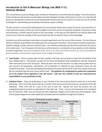
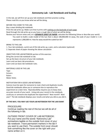
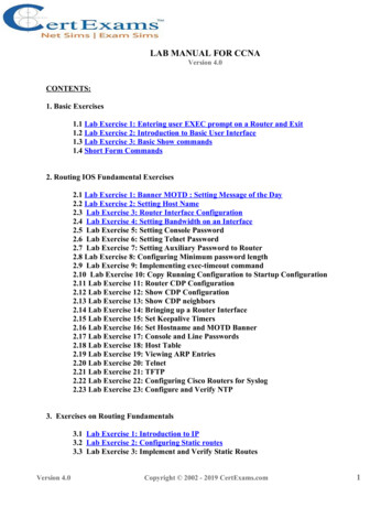
MODFLOW Lab 19: Application of a Groundwater Flow Model to a Water Supply ProblemAn Introduction to MODFLOW and SURFERThe problem posed in this lab was reported in Chapter 19 of "A Manual of InstructionalProblems for the U.S.G.S. MODFLOW Model," by P.F. Andersen, EPA/600/R-93/010, February1993. The details about the problem were exerpted from the chapter along with additionalcomments provided by J.S. Gierke.PurposeUtilize groundwater modeling software to forecast the pumping drawdown in a regional aquiferfor public drinking water supplyGroundwater flow models are often used in water resource evaluations to assess the long-termproductivity of local or regional aquifers. This exercise presents an example of an application toa local system and involves calibration to an aquifer test and prediction using best estimates ofaquifer properties. Of historical interest, this problem is adapted from one of the first applicationsof a digital model to a water resource problem (cf. Pinder, G.F., and G.D. Bredehoeft,"Application of the digital computer for aquifer evaluation," Water Resources Research, 4, 10691093, 1968). The specific objective was to assess whether a glaciofluvial aquifer could providean adequate water supply for a village in Nova Scotia.Objectives1)Become familiar with MODFLOW and its various input packages2)Gain experience in model calibration3)Become aquainted with model data presentation (e.g., Surfer contours)BackgroundThe aquifer is located adjacent to the Musquodoboit River, ¼-mile northwest of the village ofMusquodoboit Harbour, Nova Scotia. It is a glaciofluvial deposit consisting of coarse sand,gravel, cobbles, and boulders deposited in a U-shaped glacial valley (Figures 19.1 and 19.2). Theaquifer, which is up to 62 feet thick, is extensively overlain by recent alluvial deposits of sand,silt and clay, which act as confining beds. For the purposes of our analysis, it is assumed that theaquifer is fully confined with several zones of varied transmissivity (Figure 19.3).A pump test was conducted to evaluate the aquifer transmissivity and storage coefficient, and toestimate recharge from the river. The test was run for 36 hours using a well discharging at 0.963cubic feet per second (432 gallons per minute, gpm) and three observation wells (Figure 19.4).The test was discontinued when the water level in the pumping well became stable. Initialestimates of aquifer parameters were calculated using the Theis curve and the early segment ofthe drawdown curves for the observation wells. The results were somewhat variable, rangingfrom 1.45 ft2/s to 0.3 ft2/s, due to influence of boundary conditions (the Musquidoboit River) onthe pumping test.1
Introduction to MODFLOWMODFLOW, developed by the U.S. Geological Survey, uses the finite difference method toobtain an approximate solution to the partial differential equations that describe the movement ofgroundwater of constant density through porous material. Hydrogeologic layers can be simulatedas confined, unconfined, or a combination of confined and unconfined. External stresses such aswells, areal recharge, evapotranspiration, drains, and streams can also be simulated. Boundaryconditions include specified head, specified flux, and head-dependent flux. Packages available inMODFLOW and their major function are:Table 1: Names and descriptions of MODFLOW input packages.Package Name (.extension)Problem Set up and DefinitionBasic (.bas)Block Centered Flow (.bcf)Boundary Condition PackagesWell (.wel)Drain (.drn)Evapotranspiration (.et)River (.riv)General Head Boundary (.ghb)Recharge (.rch)Solution Technique PackagesStrongly Implicit Procedure (.sip)Slice Successive Over Relaxation (.sor)Pre-conditioned Conjugate Gradient (.pcg)Output Control (.oc)PurposeOverall model setup and executionSets up grid and material propertiesSpecified constant flux conditionHead-dependent flux condition limited to dischargeSimulate areal withdrawal of water due to E/T.Head-dependent flux condition with a maximumHead-dependent flux condition, no maximumSpecified areal flux input, e.g., infiltrationNumerical solution techniqueNumerical solution techniqueNumerical solution techniqueDirects amount, type, and format of outputProblem ScopeFor this first exercise, you are to gain experience in "using" MODFLOW and in manipulatinginput files manually. In future exercises, you will learn how to prepare input from scratch. Sohere, you will be using previously prepared input files and manipulating them just a little. This isjust an introduction, you will by no means be an expert at the end of this.Obtaining and Organizing the Input FilesTo start, create a subdirectory: modflow and then off that one another modflow/lab19. All thefiles will be placed in the lab1 subdirectory. Remember, unix is case sensitive, so it is suggestedthat you work in lower case.Access the webpage: http://www.geo.mtu.edu/ jsgierke/classes/modflow/lab19/lab19.html2
Hold the SHIFT key down while clicking on each file with the left mouse button (Sun mouse) orright mouse button (PC mouse). When a pop-up menu appears asking where to save the file,insert the subdirectory path you created above (modflow/lab19) between your root diretory andthe filename.You should have received the following data files (type ls ab19.ocRunning MODFLOWThe format of MODFLOW input files is give in Appendix A. You will use this appendixfrequently.The version of MODFLOW that you will use here is called "surfmod" and this is run by typingthe following:surfmodThe program will ask for file names according to input and output unit numbers as definedbelow:Unit 66: this is the standard MODFLOW output; the name is user specified. CAREFULL: youcan overwrite other files if you do not provide a unique filename. Call this lab19.outUnit 1: lab19.bas; this is always the basic package, which defines the unit numbers for the otherpackages. The ones listed below are unique to this problem.Unit 11: lab19.bcfUnit 12: lab19.welUnit 14: lab19.rivUnit 19: lab19.sipUnit 22: lab19.ocUnit 80: 1lay19.dat, this is a file prepared for input into Surfer contouring software. Ignore thisfile for the time being and overwrite it with each simulation during the calibration phase below.Run the model with these given data sets (a summary of the input is given in Table 19.1). Plotthe drawdowns (using either an Excel or Applix spreadsheet) the observation wells and compareto the field data listed in Table 19.2. Manipulate the value of the Transmissivity Multiplierand/or the Storativity (both can be found in lab1.bcf) until you are satisfied with the results.(Hint: It is pretty easy to edit lab1.bcf with the vi or pico editors, save it, and rerun surfmod. Usedifferent names for the Unit 66 file for each run so that you can save them and zero in on the3
best values of T & S.) Print out the graph with the "best" fit. You might as well know now thatthere is no combination of S and T that will yield an exact agreement. In fact, you will be able tomatch either the early time data ( 100 minutes) or the later time data ( 100 minutes) but notboth unless you use time-variable storage coefficient, which is beyond the scope of this lab. Sofit the part you want realizing that you are calibrating to the pumptest data with the purpose of"forecasting" drawdowns for even longer times (see below).Once you have calibrated S and T, now run a simulation for 1000 days by altering the value ofPERLEN in lab1.bas (the units are seconds) and NSTEPS (increase to 30, if not already set to30). Using Surfer and 1lay19.dat, draw a drawdown contour for the aquifer region at 1000 days(the data for this is the last 2420 lines of data in the file 1lay19.dat).Examine the water budget calculations at the end of the best fit simulation (36-hrs) and the 1000day simulation. Compare where the water is coming from between these two times.Introduction to SurferThe Surfer program is designed to generate contour plots of inputted data by three differentmethods (see Appendix B for a little more details): inverse distance, kriging, or minimumcurvature. Inverse distance is an averaging method that weights data values such that theinfluence of a data point decreases with the distance from the grid value being generated. Krigingperforms a moving average that defines trends in the data. High points in the same region of themap tend to be connected as ridges, or low points connected as troughs. Minimum curvaturegenerates the smoothest surface of the three methods, however, data may not support the trendsas shown. Surfer can also utilize MODFLOW output to generate drawdown contour maps. In thisway, Surfer allows a visual representation of the effects of pumping on a hydrogeologic system.What to Hand inA spreadsheet plot of the model-simulated drawdowns compared to the observed drawdowns.Use good technical labelling practices.A contour plot for the 1000-day drawdown and use good technical labelling practices.A memo containing the following sections: (1) Background (simply reference the lab handout forthe background information); (2) Objectives; (3) Approach (i.e., what did you use as a model,what parameters were calibrated and how); (4) Results and Discussion (Describe the calibrationresults and the contour plot, is the system at steady state at 1000 days, why or why not (use thewater budget results)?, comment on weaknesses of and/or limitations to the calibration).4
Table 19.1. Input date for the water supply problemGrid:Grid Spacing:Initial Head:Transmissivity:Storage Coefficient:Closure Criterion:Number of Time Steps:Time Step Multiplier:Length of Simulation:Production Well Location:Pumping Rate:River Stage:River Conductance:River Bottom Elevation:44 rows, 55 columns, 1 layerUniform 100 ft0.0 ftNon-uniform spatially, 3 zonesUniform spatially0.001101.41436 hoursRow 29, column 320.963 ft3/s (432 gpm)0.0 ft0.02 ft2/s-10 ftTable 19.2. Observed drawdown data from aquifer testTime (min)141040100400100020003000Well 10.170.260.330.480.570.790.991.191.33Drawdown (ft)Well 20.040.120.160.220.290.510.700.860.985Well 30.000.010.020.080.140.300.500.680.78
6
7
Groundwater flow models are often used in water resource evaluations to assess the long-term productivity of local or regional aquifers. This exercise presents an example of an application to a local system and involves calibration to an aquifer test and prediction using best estimates of aquifer properties.