WIXLIB

T.J. Edwards et al.NeuroImage 217 (2020) 116868animals from 13 litters; of these, 10 brains of each callosal phenotype(complete CCD, partial CCD and normal CC) were scanned utilizing thefull scanning protocol described below.coherence of EEG signal between the putatively connected regions,indicating that it may mediate functional connectivity (Lazarev et al.,2016). Paradoxically, the anomalous tracts that constitute the proposedcore features of structural connectivity in human CCD have only beenidentified in a minority of cases. This is likely due to a combination offactors, not limited to: genetic heterogeneity, environmental influencesand methodological challenges of studying in vivo structural connectivityin humans.Animal models have historically been used to address some of thesechallenges, as they present an opportunity to study brain connectivity ina more controlled system. However, while the incidence and nature ofaberrant structural connectivity has been studied in humans, it has notbeen fully characterized in mouse models (Olavarria and Van Sluyters,1995; Dodero et al., 2013; Vega-Pons et al., 2017). Very few cases ofpartial CCD in mice have been described, which has to date precluded thedevelopment of a mouse model to study aberrant connectivity throughthe callosal remnant in partial CCD (Edwards et al., 2014). The establishment of such a mouse model is critical to replicate and validateanalogous connectivity changes to those in humans in a system wherehistological tract tracing is possible, and therefore to aid development ofpredictive diagnoses and therapeutic interventions.The purpose of the present study was to conduct a systematic investigation and comparison of changes in connectivity in mouse models ofboth complete and partial CCD. To this end, we backcrossed wild typeC57Bl/6J mice twice to complete CCD BTBR Tþ tf/J (BTBR) mice togenerate BTBR x C57Bl/6 N2 (BTBR N2) littermates that display eitherfull corpus callosum, complete or partial CCD (Jones-Davis et al., 2013).High resolution ex vivo diffusion MRI (dMRI) and tractography wasemployed to mathematically model the axonal connections betweenspatially separated cortical regions; these connectivity maps were in turnused to reconstruct the topological organization of the large-scale brainnetworks (or connectomes) found in both complete and partial CCD mice.These networks were subsequently compared by utilizing whole networkgraph theory measures and network-based statistics (NBS) to identify keydifferences between callosal conditions (Zalesky et al., 2010). Byapplying methods similar to those previously used to characterize humanCCD to a mouse strain with CCD, differences in structural connectivitywere identified that resemble those observed in humans. Crucially, wewere able to validate our tractography findings by in utero electroporation and immunohistochemistry, providing strong evidence for structuraldevelopmental plasticity in the mouse CCD brain. Our findings establisha mouse line with variable degrees of callosal malformations as a modelfor investigating the variability, plasticity and function of changes instructural connectivity across humans and mice with CCD.2.2. Data acquisitiondMRI volumes were acquired for complete CCD, partial CCD, andnormal CC mouse brains (n ¼ 10 for each condition). Prior to scanning,each brain was immersed in Fomblin Y-VLAC oil (Y06/6 grade, Solvay,USA); air was actively removed from each sample via vacuum pumping.Scanning was conducted using a 16.4 T vertical bore, small animal MRIsystem (Bruker Biospin, Rheinstetten, Germany; ParaVision v5.0)equipped with Micro 2.5 imaging gradient and a 15 mm linear, surfaceacoustic wave coil (M2M, Brisbane, Australia). Parameters for the dMRIspin-echo pulse sequence were as follows: matrix size (MTX) 196 114 84, field of view (FOV) 19.6 11.4 8.4 mm (0.10 mm isotropicvoxels), repetition time/echo time (TR/TE) 200/23 ms, δ/Δ 2.5/12 ms. Azero-interpolation filling factor of 10% was used across the phase andslice encoding directions. One brain was imaged at a higher resolution of0.075 mm in the anteroposterior dimension, and was resliced to 0.10 mmisotropic resolution prior to subsequent analysis. For each dataset, two b0(b-value ¼ 0 s mm 2) images and 30 diffusion-weighted (b-value ¼ 5000s mm 2) volumes were acquired. The 30 diffusion-gradient directionsused were evenly distributed over a hemisphere using the electrostaticrepulsion method. No image averaging was used. Total acquisition timewas approximately 14.5 h per brain. In addition to dMRI, each brain wasalso imaged with the FLASH imaging protocol to obtain structural imageswith the following parameters: MTX 654 380 280, FOV 19.6 11.4 8.4 mm (0.03 mm isotropic voxels), TR/TE 50/12 ms, flip angle of 30 .No image averaging was used. Acquisition time was 0.7 h per brain.Data processing was performed on a high-performance computingcluster with 1600 CPU cores and 8 TB of RAM housed at the QueenslandBrain Institute. Following image reconstruction and orientation, b0 volumes were averaged and used to generate a binary brain mask. Scalardiffusion metric images were generated via weighted least-squaresdiffusion tensor estimation, using DTIFIT from the FSL software package (Behrens et al., 2003) (FSL v 5.0; https://fsl.fmrib.ox.ac.uk/fsl/fslwiki). Color fractional anisotropy (FA) maps were generated by theproduct of primary eigenvector of the diffusion tensor and FA. Fiberorientation distribution (FOD) was estimated with MRtrix (v0.2.7; www.nitrc.org/projects/mrtrix) by constrained spherical deconvolution (CSD)using a similar procedure to those previously described (Liu et al., 2016).Briefly, a mask of high anisotropy voxels was obtained by eroding a binary mask of a fractional anisotropy map; masked voxels were subsequently thresholded at an intensity of 0.7. Voxels that survived erosionand thresholding were assumed to represent a single fiber mask, whichwas subsequently used to estimate the response function spherical harmonic coefficients with a maximum harmonic order (lmax) ¼ 6.2. Materials and methods2.1. AnimalsBreeding and experimental protocols were approved by The University of Queensland Animal Ethics Committee and were performed according to the Australian Code of Practice for the Care and Use of Animalsfor Scientific Purposes. Mice used in this study were generated byreciprocal crosses between BTBR and C57BL/6J inbred mouse strains. F1females were crossed with BTBR males to generate littermates (BTBR N2)with varying degrees of CCD. For all MR imaging, at postnatal days (P)80–82, mice were anesthetized and transcardially perfused with 0.9%saline, followed by 4% paraformaldehyde (PFA). Brains were postfixed in4% PFA for at least 48 h before storage in phosphate buffered saline (PBS)with 0.2% sodium azide. Brains were dissected from the skull andincubated in PBS with 0.2% gadopentetate dimeglumine (Magnevist,Berlex Imaging, Wayne, NJ, USA) for four days prior to imaging. Tofurther characterize the neuroanatomy of the BTBR N2 mouse (Jones-Davis et al., 2013), prior to full brain structural imaging, each brain wasscanned using a single diffusion direction to identify the callosalphenotype. In total, corpus callosum length was measured in n ¼ 1122.3. Reference atlas construction and registrationSegmentation was performed by combining two previously established ex vivo MRI-based adult mouse brain atlases: a cortical atlas fromthe Centre for Advanced Imaging at The University of Queensland (CAIatlas) (Ullmann et al., 2013), and a subcortical atlas created by the lab ofProf. Susumu Mori of Johns Hopkins University (JHU atlas) (Chuanget al., 2011). The methods used to combine the two atlases have beendescribed previously (Liu et al., 2016). Briefly, the JHU atlas wasspatially transformed to the CAI template with affine transformationfollowed by nonlinear deformation by Advanced Normalisation Tools(ANTs; http://stnava.github.io/ANTs/). Small, functionally related areaswere combined for a total of 76 regions (38 regions per cerebral hemisphere); the components of each region are summarized in Table 1 andshown in Fig. 1). To minimize areal overlap due to differences in brainregistration and partial volume effects at dMRI resolution, the perimeterof each cortical area was eroded by two voxels. Preliminary analysis of2

T.J. Edwards et al.NeuroImage 217 (2020) 116868connectivity in partial CCD and complete CCD brains identified spuriousinterhemispheric streamlines that skipped across the longitudinal fissure.To prevent this from affecting the final estimation of connectivity, a fivevoxel-wide (0.5 mm) exclusion region of interest (ROI) was manuallydrawn at the telencephalic midline between the hemispheres.A virtual callosotomy was also conducted for comparative purposes,the rationale for which has been previously discussed in-depth by Owenand colleagues (Owen et al., 2013a,b). In brief, virtual callosotomiesintroduce an additional series of controls lacking callosal connections,which can be compared with CCD brains, and allows for the differentiation of network differences in CCD brains attributable to absence ofcallosal fibers as opposed to novel connectivity outside of the CC. Thisassists in attributing differences in connectivity and network characteristics in CCD, compared to normal CC controls, to the reorganization ofconnections rather than just the absence of callosal connectivity. Thevirtual callosotomies were performed by manually drawing a midsagittalexclusion ROI over the CC in the native diffusion space of normal CCbrains. The averaged b0 volume of the dMRI volume of each brain wasmapped to the 0.1 mm isotropic adult mouse brain model by affine anddiffeomorphic transformation using the “greedy symmetric normalisation model” in ANTs; symmetric cross-correlation was used as a similarity metric with a maximum of 60 180 40 iterations (Avants et al.,2011). The inverse transformation was applied to the reference atlas tobring anatomical labels into the individual image space of each brain.Table 1Areas defined in the adult mouse brain atlas.AreaAbbreviationComponents (if applicable)SubiculumSubEntorhinal cortexEntPresubiculum, Parasubiculum, Dorsalsubiculum, Postsubiculum, Subiculumtransition areaMedial entorhinal cortex, Caudomedialentorhinal cortex, Dorsal intermediateentorhinal cortex, Dorsolateralentorhinal cortex, Ventral intermediateentorhinal cortexDorsolateral orbitalcortexFrontal associationcortexLateral orbital cortexPrimary motor cortexSecondary motorcortexVentromedial orbitalcortexParietal condarysomatosensorycortexPrimary auditorycortexSecondary auditorycortexTemporal associationareaPrimary visual cortexS22.4. Probabilistic tractography and connectome constructionA1Secondary visualcortex lateralSecondary visualcortex mediolateralV2lAnterior cingulateAcRetrosplenial areaInsular cortexEctorhinal cortexPerirhinal cortexClaustrumRsInEctPrClEndopiriform nucleusEndPiriform nucleusPirAmygdalaAmHippocampusCaudate putamenLateral globuspallidusOlfactory bulbAccumbens nucleusHypothalamusSeptumThalamusSuperior colliculusInferior colliculusPeriaqueductal greyCerebellumHpCpLgpCSD-based probabilistic tractography (using the SD PROB algorithm)was performed using in-house scripts based on MRtrix (v0.2.7) (Tournieret al., 2012) using procedures similar to those described previously(Moldrich et al., 2010; Liu et al., 2016). The tractography tracking parameters were as follows: FOD cut-off ¼ 0.1, maximum number of 10,000streamlines, maximum number of attempts ¼ 1,000,000, step size ¼ 10μm, curvature threshold ¼ 11.5 /step, minimum/maximum streamlinelength ¼ 0.5/20 mm. Probabilistic tractography was initiated from eachcortical and subcortical anatomic label. Whole brain connectivitymatrices were generated using a two-step approach; first, streamlineswere seeded from each atlas-based region and the fraction of the totalnumber of streamlines passing through each voxel relative to the totalnumber generated was used to create a connectivity map for each seedregion (76 tractography results). The connectivity map of each seed wasmasked by each of the remaining 75 anatomic labels; a putativeconnection between a pair of regions was retained for further analysiswhen the average of the ratio between the sum of connected voxel valuesand the volume of the region was greater than zero. Next, tractographybetween each pair of potentially connected regions identified in the firststep was performed whereby both anatomic labels were specified as“seed” and “include” regions for streamline generation. The samethreshold was applied to the resulting tractography results and the surviving connections were entered into a 76 76 connectivity matrix foreach brain. For subsequent analysis of connectomes, connections werefurther weighted by the mean FA across voxels assigned a connectivityvalue greater than 0.001 for each area pair combination; consequently,the connection ‘strength’ between cortical regions was also weighted bythe tissue microstructural features of the neural tract connecting themgenerated by tractography, rather than within the atlas-defined area.FraLoM1M2VmoPaA2Medial orbital cortex, Ventral orbitalcortexLateral parietal association cortex,Medial parietal association cortex,Parietal cortex, posterior area, rostralpartPrimary somatosensory cortex, barrelfield, dysgranular zone, forelimb region,hindlimb region, jaw region, shoulderregion, trunk region, upper lip regionSecondary auditory cortex dorsal area,Secondary auditory cortex ventral areaTaV1V2mlPrimary visual cortex, Primary visualcortex binocular area, Primary visualcortex monocular areaSecondary visual cortex mediomedialarea, Secondary visual cortexmediolateral areaCingulate cortex area 24a, 24a0 , 24b,24b0 , 25, 32Cingulate cortex area 29a, 29b, 29c, 30Claustrum, Claustrum dorsal part,Claustrum ventral partDorsal nucleus of the endopiriform,Intermediate nucleus of theendopiriform claustrum, Ventral nucleusof the endopiriform claustrumCortex-amygdala transition zones,Piriform cortex, Amygdalopiriformtransition area, Rostralamtydalopiriform areaPosterolateral cortical amygdaloid area,Posteromedial cortical amygdaloid areaObAnHypSepThalScIcPagCb2.5. Connectome visualizationConsensus connectomes were constructed for each condition: complete CCD, partial CCD, normal CC and virtual callosotomy controls.Connections present in half of the individual connectomes of each groupwere included in the consensus connectome and connection strength(based on FA) was averaged across all brains. Connectomes were visualized in anatomical layouts or circular layouts constructed using theBrainNet Viewer visualization tool (https://www.nitrc.org/proj3

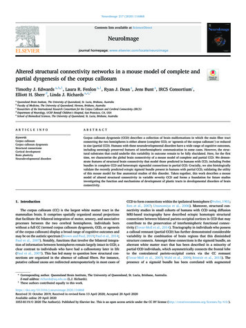
T.J. Edwards et al.NeuroImage 217 (2020) 116868Fig. 1. 3D representation of the adult mouse brain atlas.Each colour indicates a distinct ROI in the atlas, corresponding to the areas outlined in Table 1, in horizontal (A), sagittal (B) and coronal (C) views.callosal conditions. The participation coefficient was calculated by utilizing the previously determined consensus community partitions, asdescribed previously (Guimer a and Amaral, 2005), and were displayedusing the Gephi toolkit (Bastian et al., 2009).ects/bnv/) (Xia et al., 2013) and Circos software (https://www.cpan.org/ports; Krzywinski et al., 2009), respectively. For anatomical layouts, nodes were plotted at the center of gravity for each atlas region(calculated using the center of gravity function in FSL) and colored according to degree using a custom colormap. Edges between nodes wereweighted according to mean FA across the tract. A complete descriptionof the methods used to generate circular connectomes, also known asconnectograms, is outlined by Irimia et al. (2012). Briefly, atlas regionswere represented as uniquely colored radially oriented segments, ordered according to lobe assignment, and separated into left and righthemispheres. Within each lobe, parcellations were arranged approximately according to the order of their location along the dorso-ventralaxis. Individual node measures were calculated by methods describedin the following section, averaged across all individual brains for eachcondition, and displayed in concentric radially oriented segments fromoutside in: node strength, local efficiency, betweenness, clustering, andmodule assignment. Edges are weighted according to the streamlinecount for each pairwise area connection and are colored according tomean FA across the tract (red ¼ top tertile, green ¼ middle tertile, blue ¼bottom tertile).2.7. StatisticsAll statistical comparisons were performed using the GraphPad Prismsoftware package (v 7.0a for Mac, GraphPad Software, La Jolla CaliforniaUSA). Statistical comparisons between the AUC of all measures wereperformed using unpaired two-tailed Student’s t-tests with Holm-Sidakcorrection for multiple comparisons and a threshold for significance ofp 0.05. Normality of distribution of indicated datasets was assessed viaD’Agostino-Pearson omnibus normality tests and differences in varianceof datasets was probed with F tests (significance cut-off p 0.05). To testif individual networks were more or less similar to other individualnetworks in both complete and partial CCD compared to controls, theaverage edge-wise correlation coefficient between each pair of brainswithin each callosal condition was calculated. The nine averaged valuesobtained for each network (i.e. ten comparisons excluding the correlationof a network with itself) were averaged to obtain a measure of similarityof each individual network to other individual networks with the samecallosal condition. These values were calculated across the wholenetwork, and for interhemispheric and intrahemispheric connectionsseparately, to determine the relative contribution of both to overallvariability.To identify subnetworks of connections that differed significantlybetween callosal conditions, the NBS toolbox was utilized (Zalesky et al.,2010). The NBS controls for the family-wise error rate (FWER), whichwould normally complicate comparisons of every connection in anetwork, by performing permutation testing on connected graph components comprised of a set of connections that reach an initialtest-statistic threshold. Graph components that reached p 0.05(FWER-corrected) were considered to be significantly different betweenconditions (number of permutations ¼ 5000, tested across a range ofinteger thresholds between 2 and 5). Due to the variability in CCD connectomes, an additional discovery strategy was employed to identifynovel and preserved individual connections in partial CCD. In this case,novel connections were defined as network edges that were present intwo or more brains per condition (i.e. 20% penetrance), but did not existin any normal CC brain.2.6. Network and node-based analysisComparisons of graph theory measures at the network and node levelof structural connectomes were performed using GRETNA (Wang et al.,2015) (https://www.nitrc.org/projects/gretna/). All networks wereproportionally thresholded based on sparsity in GRETNA (Wang et al.,2015), using thresholds ranging from 0.05 to 0.13 (incrementing in stepsof 0.01), to exclude weak or spurious connections while simultaneouslymaintaining the same network density across all tested conditions. Meannodal strengths, mean nodal betweenness, network global efficiency,mean nodal local efficiency and mean nodal clustering coefficient werecalculated for each connectome for each threshold level, as well as theircorresponding area-under-the-curve (AUC) across the full thresholdrange.The strength of a node was defined as the sum of the weights of theedges directly connecting that node to another, ‘neighboring’, node; thestrengths of all nodes in a connectome were averaged to obtain the meanweighted degree of the network. The betweenness of a node was definedas the percentage of all shortest paths between each pair of nodes in anetwork that contains that node (Brandes, 2001). Mean betweenness wascalculated by averaging the betweenness of all nodes in the network.Global efficiency was defined as the inverse of the mean path lengthbetween all nodes in the network. Local efficiency was defined analogously, but for local neighborhoods of nodes. The clustering coefficientwas defined for each node as the ratio of neighboring nodes that are alsonodes of each other (Watts and Strogatz, 1998). For all measures, calculations were made on weighted edge measures based on the average FAvalue as described in the preceding section, and the AUC for all thresholds was calculated.The modularity of each network was determined by the brain connectivity toolbox implementation of the Louvain community detectionalgorithm (Rubinov and Sporns, 2011). Gamma was optimized formodularity for normal CC controls (γ ¼ 1.2), which was applied to other2.8. ROI-based tractography analysisTractography and functional imaging studies in CCD humans havesuggested that alternative commissures in the midbrain and forebrainmay compensate for the absence of callosal fibers (Tovar-Moll et al. 2007,2014; Tyszka et al., 2011, Lazarev et al., 2016). To determine the specificconnectivity of alternative commissures in BTBR N2 mice we performedROI-based tractography of the anterior commissure, posterior commissure, hippocampal commissure and CC. To determine the connectivity ofthese tracts, ROIs were drawn bilaterally in two parasagittal planes,approximately 0.3 mm to the left and right of the midsagittal plane, in thediffusion image space of each individual brain. These ROIs were then4

T.J. Edwards et al.NeuroImage 217 (2020) 1168682.11. Histological image acquisition and data analysisused to generate streamlines for each commissure using identical parameters to those used to generate structural connectomes, with 50,000streamlines selected for each tract before tracking was terminated. Individual tractography results were converted to connectivity maps bycalculating the fraction of streamlines passing through each voxel as aproportion of the total number of streamlines generated. The resultingconnectivity maps were each warped to the common atlas space usingwarps generated in the process of atlas registration, and were thenaveraged across the 10 animals in each condition to produce a singlemean streamline density map of each condition. To reconstruct heterotopic tracts, tractography was seeded from the frontal association cortex.Inclusion ROIs were specified as bilateral parasagittal callosal ROIs, andthe ipsilateral frontal and contralateral occipital projections of the CC.Exclusion ROIs were specified as the midline exclusion ROI specified bythe brain atlas, as well as contralateral frontal and ipsilateral occipitalprojections. CSD-based probabilistic tractography was performed withthe following parameters: FOD cut-off ¼ 0.2, maximum number of 10,000 streamlines, maximum number of attempts ¼ 1,000,000, step size ¼10 μm, curvature threshold ¼ 11.5 /step, minimum/maximum streamline length ¼ 5/40 mm.At least 10 sections throughout the dorsolateral extent of each brainwere carefully examined and each animal categorized as control, partialor complete CCD using the criteria of: 1. the presence or absence of anycallosal fibers; 2. the presence or absence of complete or partial Probstbundles and; 3. the size of the callosal tract at the midline. Any brains thatwere considered a borderline case for any of these three criterion wereexcluded from further analysis. Ten animals that clearly satisfied thecontrol criteria and ten that satisfied the partial CCD criteria that hadcomparable size and location of fluorescent transfected fields and wereage-matched were selected for further analysis. Sections were matched inthe dorso-ventral position across individual brains prior to analysis. Highresolution confocal images were acquired of the contralateral frontalcortex (ROI 1 and 2) and contralateral homotopic cortex (ROI 2) using aDiskovery spinning disk confocal microscope (Spectral AppliedResearch) with two cCMOS cameras (Andor Zyla 4.2) and a 20x/0.75 NAair objective (Nikon) controlled with Nikon NIS software. Widefieldimages of entire sections were acquired with a Zeiss upright Axio-ImagerZ1 microscope fitted with Axio-Cam HRm camera and captured with Zensoftware.2.9. In utero electroporation and tissue collection2.12. Analysis of histological imagesIn utero electroporation of embryos and postnatal tissue collection forhistological validation of ectopic tracts was performed as describedpreviously (Kozulin et al., 2016; Su arez et al., 2014; Fenlon et al., 2017).In brief, F1 females were placed in the same cage as BTBR males overnight and where a vaginal plug was detected on the next day, this wasconsidered embryonic day (E)0. For electroporation surgery, pregnantdams were anesthetized with an intraperitoneal injection of ketamineand xylazine (120 mg/kg ketamine; 10 mg/kg xylazine) at E15, when inutero electroporation is well established to predominantly label layer 2/3neurons of the cortex (Su arez et al., 2014). Dams underwent a lapa

umes were averaged and used to generate a binary brain mask. Scalar diffusion metric images were generated via weighted least-squares diffusion tensor estimation, using DTIFIT from the FSL software pack-age (Behrens et al., 2003) (FSL v 5.0; https://fsl.fmrib.ox.ac.uk/fsl/fs lwiki). Color fractional anisotropy (FA) maps were generated by the