Energy Budget-based Backscatter In An Eddy Permitting Primitive . PDF Free Download

1y ago

30 Views

1 Downloads

2.52 MB

12 Pages

Report/dmca

Download PDF

Transcription

Ocean Modelling 94 (2015) 15–26Contents lists available at ScienceDirectOcean Modellingjournal homepage: www.elsevier.com/locate/ocemodEnergy budget-based backscatter in an eddy permitting primitiveequation modelMalte F. Jansen a,b,c, , Isaac M. Held b,c, Alistair Adcroft b,c, Robert Hallberg b,caDepartment of the Geophysical Sciences, The University of Chicago, Chicago, IL 60637, USANOAA Geophysical Fluid Dynamics Laboratory, Princeton, NJ 08540, USAcProgram in Atmospheric and Oceanic Sciences, Princeton University, Princeton, NJ 08540, USAba r t i c l ei n f oArticle history:Received 15 April 2015Revised 3 July 2015Accepted 22 July 2015Available online 31 July 2015Keywords:BackscatterEddy parameterizationMesoscaleEddy-permittingEnergy budgetNegative viscositya b s t r a c tIncreasing computational resources are starting to allow global ocean simulations at so-called “eddypermitting” resolutions, at which the largest mesoscale eddies can be resolved explicitly. However, an adequate parameterization of the interactions with the unresolved part of the eddy energy spectrum remainscrucial. Hyperviscous closures, which are commonly applied in eddy-permitting ocean models, cause spurious energy dissipation at these resolutions, leading to low levels of eddy kinetic energy (EKE) and weak eddyinduced transports. It has recently been proposed to counteract the spurious energy dissipation of hyperviscous closures by an additional forcing term, which represents “backscatter” of energy from the un-resolvedscales to the resolved scales. This study proposes a parameterization of energy backscatter based on an explicit sub-grid EKE budget. Energy dissipated by hyperviscosity acting on the resolved ﬂow is added to thesub-grid EKE, while a backscatter term transfers energy back from the sub-grid EKE to the resolved ﬂow. Thebackscatter term is formulated deterministically via a negative viscosity, which returns energy at somewhatlarger scales than the hyperviscous dissipation, thus ensuring dissipation of enstrophy. The parameterization is tested in an idealized conﬁguration of a primitive equation ocean model, and is shown to signiﬁcantlyimprove the solutions of simulations at typical eddy-permitting resolutions. 2015 Elsevier Ltd. All rights reserved.1. IntroductionThe ocean circulation is strongly controlled by mesoscale turbulent eddies (e.g. Gill et al., 1974; Johnson and Bryden, 1989; Hallbergand Gnanadesikan, 2006; McWilliams, 2008; Waterman et al., 2011).However, most of the current generation climate models, as for example appeared in the report of the Intergovernmental Panel on Climate Change (IPCC; Flato et al., 2013), have too little spatial resolutionto resolve these turbulent motions. The effect of unresolved turbulent motions on the larger-scale resolved ﬂow thus must be parameterized. Since any such parameterization is associated with uncertain assumptions about the properties of the eddies, many modelinggroups aim to increase the resolution of their ocean climate modelssuch as to resolve eddies explicitly. In the near future we expect theresolution of many IPCC-class ocean models to be reﬁned to around1/4 of a degree. These resolutions are often considered “eddy permitting”, because the models produce eddy-like disturbances generated by baroclinic instability of the ﬂow, but the resolution is still Corresponding author at: Department of the Geophysical Sciences, The Universityof Chicago, Chicago, IL 60637, USA. Tel.: 1 617 230 0262.E-mail address: mfj@uchicago.edu (M.F. .0151463-5003/ 2015 Elsevier Ltd. All rights reserved.insuﬃcient to properly resolve the mesoscale eddy ﬁeld (e.g. Hallbergand Gnanadesikan, 2006; Hallberg, 2013). It therefore remains important to devise parameterizations that adequately describe sub-grideddy effects at these eddy-permitting resolutions.The qualitative properties of the mesoscale eddy ﬁeld in the oceancan be understood by considering the quasi-geostrophic (QG) approximation (Charney, 1971; Rhines, 1977; Salmon, 1978). A fundamentalproperty of QG turbulence is the transfer of enstrophy (i.e. vorticityvariance) to smaller and smaller scales, by non-linear eddy-eddy interactions (Charney, 1971). In an ocean model where only part of themesoscale eddy kinetic energy (EKE) spectrum is resolved, enstrophy must be removed near the grid-scale to represent the net transfer of enstrophy to the subgrid-scale, and avoid accumulation. Thisis commonly achieved by a horizontal hyper-viscosity—typically biharmonic (i.e. fourth order)—which scale-selectively removes enstrophy near the grid-scale (e.g. Böning and Budich, 1992; Griﬃes andHalberg, 2000; Oschlies, 2002; Fox-Kemper and Menemenlis, 2008).However, at “eddy permitting” resolutions, where the grid-scale is onthe same order as the ﬁrst baroclinic deformation radius, such closures dissipate not only enstrophy, but also a signiﬁcant amount ofenergy (e.g. Jansen and Held, 2014). This energy dissipation is notdesired, since QG turbulence generally does not transfer energy to

16M.F. Jansen et al. / Ocean Modelling 94 (2015) 15–26Fig. 1. Interface height (thick grey line) and associated geostrophic velocity (black contours—contour interval: 0.5 cm/s) for the equilibrium solution of the interface-heightrestoring forcing. Notice that, in the absence of horizontal momentum ﬂuxes (required to balance frictional drag in the vertically integrated zonal mean zonal momentum budget),there is no ﬂow in the lower layer.smaller scales in the net, and thus does not provide a pathway toenergy dissipation at small scales. As a result of this spurious viscous energy dissipation, eddy-permitting models typically have toolittle EKE and too weak eddy induced transports (e.g. Hallberg, 2013;Jansen and Held, 2014; Griﬃes et al., 2015).Jansen and Held (2014) recently proposed to combine a hyperviscous closure with a forcing term, which is chosen such as to cancelthe spurious energy dissipation associated with the hyperviscosity,while maintaining a net dissipation of enstrophy. A similar approachhas also been proposed independently by Thuburn et al. (2014), whoshow improvements in simulations of barotropic turbulence. Theforcing term may be thought of as representing back-scatter of kinetic energy from the subgrid scales to the resolved ﬂow (see e.g.Kraichnan, 1976; Leith, 1990; Frederiksen and Davies, 1997; Duanand Nadiga, 2007; Kitsios et al., 2013; Grooms et al., 2015; Berloff,2015). Jansen and Held (2014) test two different formulations for thebackscatter term in a two-layer QG model, one stochastic and one deterministic. Either approach is shown to greatly improve the resultsof simulations at eddy permitting resolutions.In this paper we formulate a parameterization based on the argument of Jansen and Held (2014) for a primitive equation ocean model.The main additions to the results discussed in Jansen and Held (2014)are the implementation in a primitive-equation ﬁnite-volume model(the simulations in Jansen and Held (2014) employed a QG pseudospectral model), as well as the formulation of a local prognostic subgrid EKE budget, which is necessary to adequately account for spatialinhomogeneities in the eddy ﬁeld. The backscatter from the sub-gridEKE to the resolved ﬂow will be formulated similarly to the deterministic approach in Jansen and Held (2014) using a negative Laplacianviscosity. A similar approach has also been found to be successful inthe barotropic turbulence simulations of Thuburn et al. (2014), and issupported by the theoretical results of Kraichnan (1976) and Galperinet al. (1993).2. Resolution dependence of numerical simulationsIn the following section we discuss results from a series of numerical simulations, using an idealized two-layer conﬁguration ofthe GOLD ocean model (Hallberg, 2013; Hallberg and Adcroft, 2009).The model setup is described in Section 2.1. In Section 2.2 we discuss properties of the emerging turbulent ﬂow and their dependenceon the horizontal resolution. Consistent with the results of Jansenand Held (2014), simulations at eddy-permitting resolution will beshown to have too little EKE, as well as too weak eddy-driven meanﬂows. The purpose of the backscatter parameterization, discussed inSection 3, is to alleviate this shortcoming.2.1. Model descriptionThe numerical model setup is based on the two-layer zonally-reentrant channel conﬁguration of the GOLD ocean model discussedby Hallberg (2013), but with added topography and somewhat modiﬁed parameters, more typical of the Southern Ocean. The Cartesiancoordinate channel measures 1600 km 1600 km, and is boundedmeridionally by free slip, no-normal-ﬂow boundary conditions. TheCoriolis parameter increases from f 1.1 10 4 s 1 at the southern end of the domain to f 1.3 10 4 s 1 at the northern end ofthe domain. While motivated by the Southern Ocean, our simulations thus represent a northern hemisphere channel ﬂow. The upper layer extends on average over the upper 500 m of the 2000 mdeep domain. The zonal mean interface height is restored to a hyperbolic tangent proﬁle with a characteristic width of 500 km, on atime-scale of one year, but with no damping of departures from thezonal mean. The equilibrium solution for the interface height restoring is shown in Fig. 1. The density contrast between the two vertiρ0 7 10 4 , leading to a baroclinic gravity wavecal layers is δρ / speed of about δρ /ρ0 gH1 H2 (H1 H2 ) 1 1.6 ms 1 . The bottomtopography consists of an interrupted meridional ridge and a seamount (Fig. 2). The maximum topographic elevation is 750 m, whichis about half of the lower layer depth. Bottom friction is described viaa quadratic drag law, with a bottom-drag coeﬃcient CD 0.03. An additional background bottom velocity, U0 0.1 m/s, is included in thecomputation of the bottom drag, as a crude representation of tidalcurrents and other missing processes in the deep ocean. Enstrophyis dissipated near the grid-scale using a biharmonic viscosity, with aviscosity coeﬃcient following Smagorinsky (1963) (see Griﬃes andHalberg, 2000, for the biharmonic formulation):ν4 CSmag 4 D .(1)CSmag here is a constant non-dimensional coeﬃcient, is the gridspacing, and D (ux vy )2 (uy vx )2 is the deformation rate.

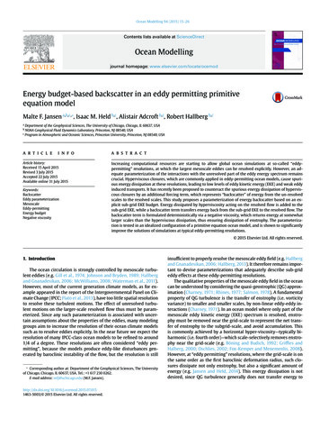
1350155017501950M.F. Jansen et al. / Ocean Modelling 94 (2015) 1750 1550600200019508001350y [km]5010001951200600800100012001400x [km]Fig. 2. Model bathymetry (depth in m—contour interval: 100 m).Unless otherwise noted, the Smagorinsky coeﬃcient is chosen similarly as in GFDL’s global ocean models: CSmag 0.06. The sensitivityof the results to CSmag will be discussed.The non-linear advection of momentum in the model is formulated in terms of a vorticity ﬂux (or generalized Coriolis) term anda KE gradient term (Hallberg, 2013). Of particular importance hereis the representation of the vorticity ﬂux term, whose discretizationimpacts the models conservation properties for kinetic energy andenstrophy. Since the energy and enstrophy budget lies at the core ofthe developed parameterization, it is desirable to choose a numericaldiscretization which by itself is approximately conservative. The numerical discretization used for this study is based on a formulationdiscussed in Arakawa and Hsu (1990). This scheme exactly conservesenergy and conserves enstrophy in the limit that the horizontal massﬂux is non-divergent.The baroclinic deformation radius varies from about 9 km at thenorthern end of the domain and above the topography, to about16 km at the southern end of the domain. Using a similar setup(though without bottom topography), Hallberg (2013) argued thatthe grid-spacing may be at most half as large as the deformation radius to adequately resolve baroclinic eddies. Simulations are here performed at varying resolutions between 3.2 km and 20 km.While 3.2 km is expected to be adequately eddy resolving, 20 km may be considered barely eddy permitting, as the grid-spacingexceeds the baroclinic deformation radius. All simulations are spunup to a statistical equilibrium for 15 years, and ﬂow statistics are averaged for 15 years following this initial spin-up period.2.2. Resolution dependenceFigs. 3 and 4 show the time-mean ﬂow and EKE for simulationsat 3.2 km, 10 km, and 20 km resolution. The highest resolution(3.2 km) reference simulation shows an overall eastward ﬂow inthe upper layer which is strongly channeled by the topographicfeatures shown in Fig. 2. The ﬂow around topography is generallyanti-cyclonic, which becomes particularly clear in the lower level,where the ﬂow is dominated by an anti-cyclone centered above thesea mount near y 1000 km. Additional localized currents emergenear the edges of the ridge around y 200 600 km. The spin-up ofanti-cyclonic ﬂows around sea-mounts is commonly known as the“Neptune effect”, and is caused by eddy PV ﬂuxes acting to reduce17the PV anomaly associated with the topography (Bretherton andHaidvogel, 1976; Holloway, 1992; Greatbatch and Li, 2000). StrongEKE is found mostly between about y 500 km and y 1300 km. Itis largest down-stream of the topographic features—particularly inthe lee of the sea mount—and weaker right above the topography.At a resolution of 10 km the EKE is signiﬁcantly reduced,though the overall spatial pattern remains largely similar. Changes inthe mean ﬂow are larger in the lower layer, which shows a weakeningof the topographically induced ﬂow. Since this ﬂow is driven by eddyﬂuxes of PV, the weakening of the topographic mean ﬂow is expectedas a result of the reduced EKE. At 20 km the EKE is much tooweak, resulting in weak topographically steered ﬂows in the lowerlayer. Changes in the upper layer mean ﬂow are less dramatic, but theﬂow becomes signiﬁcantly more zonally symmetric, and more conﬁned to the region between y 400 km and y 1200 km, thus moreclosely resembling the equilibrium solution of the restoring (Fig. 1).Additional simulations were performed at horizontal resolutionsof 5 km and 32 km (not shown). The results obtained at 5 kmresolution differ relatively little from those at 3.2 km resolution,suggesting that the large-scale ﬂow ﬁeld is mostly converged atthis resolution. This is in agreement with the numerical results ofHallberg (2013), as well as with the theoretical discussion in Jansenand Held (2014), which concluded that spurious hyper-viscous energy dissipation decreases rapidly when the grid-scale becomes smallcompared to the deformation radius. At 32 km resolution, eddies areabsent and the mean ﬂow is virtually identical to the equilibrium solution of the restoring.An important role of eddies in the ocean is to drive an overturningtransport, which releases available potential energy from the meanstate (and thus acts as the source of energy for the eddies themselves) and contributes to the transport of heat and other tracers(e.g. Johnson and Bryden, 1989; Hallberg and Gnanadesikan, 2006;McWilliams, 2008). Due to the lack of an explicit wind stress, whichwould drive an Eulerian circulation, the entire meridional overturning transport in the present model is driven by eddy ﬂuxes. The overturning transport in a statistically steady state can be computed as [v1 h1 ] [v2 h2 ] ,(2)where the overbar and brackets respectively denote the time- andzonal-average, vi is the meridional velocity in layer i, and hi is thelayer thickness. Due to the conservation of mass (or volume in theBoussinesq limit), the total transport in the two layers is equal andopposite.The overturning transport for the three simulations discussedabove is shown in Fig. 5 (solid lines). The high resolution referencesimulation (black line) shows a meridional overturning transportthat is mostly conﬁned to the strongly forced region between abouty 400 km and y 1200 km. The overturning transport peaks nearthe center of the domain at somewhat over 0.6 m2 /s. To get a better appreciation of the magnitude of the overturning transport in oursimulations, we can multiply the values in Fig. 5 by the characteristic length of the ACC: 20 000 km. This would suggest a peaktransport of around 10–15 Sv, which is on the same order as theoverturning transport in the ACC (e.g. Talley, 2013). Dividing the overturning transport by the slope of the interface yields an eddy interfaceheight diffusivity, which in turn is analogous to the GM coeﬃcientin z-coordinate models (e.g. Gent et al., 1995; Hallberg, 2013; Jansenet al., 2015). With a characteristic interface height slope near the domain center of around 500 m/500 km 10 3 , an overturning transport on the order of 1 m2 /s corresponds to an eddy diffusivity on theorder of 1000 m2 /s, which again is on the same order as suggested byobservations in the Southern Ocean (e.g. Tulloch et al., 2014).At a resolution of 10 km the peak overturning transport isreduced by about 20% relative to the high resolution simulation.The relative weakening is somewhat stronger on the ﬂanks of the

18M.F. Jansen et al. / Ocean Modelling 94 (2015) 15–26Upper LayerLower Layer 3.2 km150010001000y [km]y [km] 3.2 km15005005000205001000150001840500 10 km100015003.5 10 km16150015003105002.510002cm/s12y [km]1000cm/sy [km]1450081.56050010001500 20 km041050010001500 20 km20.51500150001000y [km]y [km]050050001000500100001500x [km]050010001500x [km]Fig. 3. Time-mean ﬂow speed (shading) and direction (arrows) for simulations with 3.2 km (top), 10 km (middle), and 20 km (bottom) resolution. The left column show the meanﬂow in the upper layer, while the right column shows the mean ﬂow in the lower layer. The color shading is identical between the three simulations, but differs between the tworespective vertical layers.overturning cell, indicating a slight reduction of the meridional extent. At a resolution of 20 km, the peak overturning transport isreduced to less than a quarter of the high resolution reference case,and the meridional extent is reduced signiﬁcantly. The results for theresolution dependence of the overturning transport largely reﬂect thereduction of EKE observed in Fig. 4.2.2.1. EKE spectra and the role of the Smagorinsky coeﬃcientTo analyze the effect of sub-grid eddy parameterizations, it is often fruitful to look at the EKE budget. For simplicity, we will here focus on the barotropic mode EKE, which arguably is most importantfor the eddy heat transport and release of available potential energy(e.g. Larichev and Held, 1995; Cessi, 2008; Jansen et al., 2015). Thespectra are deﬁned as a function of the total wavenumber asE (K ) ddK 1( ût 2 v̂t 2 ) dk dl,2(3)k2 l 2 K 2where ût and v̂t are the spectral transforms of the zonal and meridional barotropic velocity ﬁelds, respectively. The resulting spectra areshown in Fig. 6, with the solid lines denoting the three simulationsdiscussed above. The high resolution reference simulation shows apeak in the EKE spectrum at around wavenumber 8, correspondingto a wavelength of about 200 km. Below that wavenumber the spectral energy falls off with a slope near K 3 (Charney, 1971). A muchsteeper drop in EKE is found at wavenumbers higher than about 1/3–1/2 times the Nyquist wavenumber, KN π / , presumably associated with strong dissipation due to the hyper-viscous closure. A briefﬂattening of the spectrum is again found at wavenumbers just belowthe Nyquist frequency, but due to the very small amount of energy atthese scales this is unlikely to have any signiﬁcant effect.At coarser resolution the EKE level is reduced at all scales, with anoverall reduction of about 50% at 10 km and at least one orderof magnitude at 20 km (notice the logarithmic axis). As for thehigh resolution case, the spectra fall off very steeply at wavenumbershigher than about 1/2–1/3 times the Nyquist wavenumber. The steepdecline of spectral energy above the grid-scale suggests a potentially inappropriately large viscosity coeﬃcient. The (bi-harmonic)viscosity coeﬃcient was here formulated following the argumentsof Smagorinsky (1963) and Griﬃes and Halberg (2000), as discussedin Section 2.1. While this formulation is adaptive to changes in theresolution and ﬂow properties, it is deﬁned only to within the nondimensional constant factor, CSmag . The latter was chosen based onexperience with global models, where larger viscosities may be desirable either to suppress numerical noise in certain regions (such aswestern boundary currents) or to reduce the grid Reynolds numberin order to minimize numerical diffusion (Ilcak et al., 2012).To analyze the impact of reduced bi-harmonic viscosity, we repeated the eddy-permitting simulations with 10 km and 20 km, using a Smagorinsky coeﬃcient reduced by one order of magnitude, i.e. CSmag 6 10 3 . The resulting EKE spectra are shown asdotted lines in Fig. 6. As expected, the reduction of the Smagorinsky

M.F. Jansen et al. / Ocean Modelling 94 (2015) 15–26Upper LayerLower Layer 3.2 km150010001000y [km]500250050010000150040500 10 km5001500251000205001001000302y [km]150500351500cm2 /s 2y [km]100001500 10 km2001500010001505010500 20 km10001500 20 km15005150010000y [km]y [km]050002500cm /sy [km] 3.2 km150001910005000500100015000500x [km]10001500x [km]Fig. 4. Time-mean EKE for simulations with 3.2 km (top), 10 km (middle), and 20 km (bottom) resolution. The left column show the EKE in the upper layer, while the right columnshows the EKE in the lower layer. The color shading is identical between the three simulations, but differs between the two respective vertical layers.coeﬃcient leads to a considerable increase in EKE near the gridscale. Moreover, the energy level is increased also at scales muchlarger than the grid-scale. The increased EKE at larger scales is inagreement with the argument of Jansen and Held (2014), whoshowed that spurious energy dissipation near the grid-scale leads toreduced EKE levels at all scales by suppressing energy backscatter tolarger scales. However, while the EKE levels near the peak of the energy spectrum are increased, they remain about 20% too low for thesimulation with 10 km and too low by about a factor of ﬁve forthe simulation with 20 km, as compared to the high resolutionreference case.Similar improvements are found with respect to other ﬂow characteristics. The dotted lines in Fig. 5 show the overturning transportfor the simulations with reduced CSmag . As for the EKE, the overturning transports are increased relative to the simulations with thedefault Smagorinsky coeﬃcient, but they remain too low as compared to higher resolution simulations. Particularly at a resolution of 20 km, the overturning transport remains much too weak. Similar results are also found for the mean ﬂow (not shown).3. An energetically consistent backscatter parameterizationJansen and Held (2014) argue that the reduction of EKE at eddypermitting resolutions, and the associated deﬁciencies in the eddyﬂuxes and mean ﬂow properties, are primarily a result of spuriousEKE dissipation by the viscous closure. While the viscous dissipationof EKE can be minimized by using a high-order hyperviscosity anda relatively weak hyperviscosity coeﬃcient, the requirement to dissipate a certain amount of enstrophy necessarily implies a certainamount of energy dissipation, for any purely dissipative closure. Ateddy permitting resolution (i.e. when the grid scale is on the same order as the Rossby radius of deformation) this spurious energy dissipation represents a signiﬁcant part of the total EKE generation (Jansenand Held, 2014). To overcome the problem, Jansen and Held (2014)propose to combine the hyperviscous dissipation with a forcing termthat returns energy to the resolved ﬂow, and may be thought of asrepresenting “backscatter” of energy from the sub-grid scale.The closure presented in Jansen and Held (2014) is based on aglobal energy budget, and implies an assumption about spatial homogeneity of the ﬂow. This assumption is inappropriate for larger,inhomogeneous domains, such as the global ocean, or even theidealized setup used for this study. We therefore propose to combine the argument of Jansen and Held (2014) with the suggestionof Eden and Greatbatch (2008) to formulate eddy parameterizations based on an explicit predictive sub-grid EKE budget (see alsoCessi, 2008; Marshall and Adcroft, 2010; Jansen et al., 2015). The formulation of the closure is derived in the following Section 3.1, andnumerical results are discussed in Section 3.2.3.1. FormulationIn the numerical model discussed above, enstrophy and energyis dissipated near the grid scale by a bi-harmonic horizontal viscosity. The vertically averaged energy tendency of the resolved ﬂow

20M.F. Jansen et al. / Ocean Modelling 94 (2015) 15–260.70.6 3.2 km 10 km 20 km 10 km CSmag 6 x10 30.5 10 km CSmag 6 x10 3 10 km back 20 km back[m2/s]0.40.30.20.10 0.102004006008001000120014001600y [km]Fig. 5. Overturning transport (Eq. (2)) in units of m2 /s. The black line shows the high resolution reference simulation with a grid-spacing 3.2 km. Blue lines show simulationswith a resolution of 10 km, and red lines show simulations with a resolution of 20 km. The solid lines show results from the reference simulations with Smagorinsky-typebiharmonic viscosity and CSmag 6 10 2 . The dotted lines show results from simulations with a reduced Smagorinsky coeﬃcient: CSmag 6 10 3 (see Section 2.2.1). The dashedlines show results using the backscatter parameterization discussed in Section 3. (For interpretation of the references to color in this ﬁgure legend, the reader is referred to the webversion of this article.)100K 310 -1E (K )[m 3 /s 2 ]10 -210-310-410-510-610 -7 3.2 km 10 km 20 km 10 km C Smag 6 x10 -3 20 km C Smag 6 x10 -3 10 km backscatter 20 km backscatter10 010 1K [2 /L ]10 2Fig. 6. Barotropic EKE as a function of the total wavenumber, normalized by the width of the domain: K (k2 l 2 )1/2 /(2π /L). The different simulations are marked as in Fig. 5.associated with biharmonic dissipation can be computed asĖdiss1 hi Ah,i ui · ( 2 ui )H(4)iwhere hi is the thickness of layer i, H is the total depth, and Ah,i isthe biharmonic horizontal viscosity coeﬃcient, which may vary bothin the horizontal as well as between vertical layers. ui here denotesthe horizontal velocity vector and ( x , y ) the horizontal gradient. For simplicity the equations are here formulated for an isopycnallayer model, and assuming a Cartesian coordinate system, as appliesfor our idealized model setup. However, the implementation in GOLDmakes use of a generalized coordinate formulation and can thus readily be used in a global model conﬁguration (Griﬃes and Halberg,2000; Griﬃes, 2004). While not strictly negative deﬁnite, the termin (4) generally represents a sink of EKE to the resolved ﬂow.To compensate for the energy loss associated with the biharmonic viscosity, we want to include an additional forcing termin the momentum equation, which may be interpreted as representing backscatter of EKE from the sub-grid scales to the resolvedﬂow. Jansen and Held (2014) propose two formulations for this forcing term: a stochastic “noise” forcing and a (deterministic) negativeLaplacian viscosity. Both approaches were shown to be successful,

M.F. Jansen et al. / Ocean Modelling 94 (2015) 15–26with the results using negative viscosity being somewhat superior.We therefore adopt the strategy to parameterize backscatter using a negative Laplacian viscosity. While negative viscosity by itselfalso adds enstrophy to the resolved ﬂow, the proposed (energy conserving) combination of a hyper-viscous dissipation with a negativeLaplacian viscosity leads to a net dissipation of enstrophy. Negativeviscosity backscatter acts at larger scales than hyper-viscous dissipation, thus leading to a net transfer of energy from the grid-scale tolarger scales, which is associated with a net dissipation of enstrophy.Apart from being physically desirable, the net conservation of energyand dissipation of enstrophy are important for the numerical stabilityof the parameterization scheme. By bounding the energy and enstrophy norms, the approach proposed here remains numerically stabledespite the use of a negative viscosity. A more detailed discussion ofthe implications of our approach for the spectral energy and enstrophy budget, as well as for the numerical stability, is provided in Jansenand Held (2014).The effect of a Laplacian viscosity on the EKE of the resolved ﬂowcan be computed asĖback 1 ν hi ui 2 ,H(5)iwhere ν is the Laplacian viscosity coeﬃcient, which here is negativeand controls the strength of the energy backscatter. For simplicity, νis assumed constant in the vertical. We will return to the choice ofν below. Notice that there is some freedom as to how exactly thesub-grid energy source and sink terms in Eqs. (4) and (5) are formulated, with different formulations differing by contributions thatcan be absorbed into the ﬂux term. The formulations chosen herehave the advantage that they are Galilean invariant, the backscatteris positive deﬁnite, and there exists a certain symmetry between thehyper-viscous and backscatter terms—speciﬁcally the two terms arein phase for plane waves.The resolved ﬂow EKE tendencies associated with the biharmonicviscosity and backscatter are interpreted as energy exchanges withthe unresolved ﬂow, which suggests a sub-grid EKE budget equationof the form t e Ėdiss Ėback 1 ·F DH(6)where e is the vertically averaged sub-grid EKE, F denotes a horizontal ﬂux of sub-grid EKE and D denotes dissipation. Recall that Ėdiss isgenerally negative, from its deﬁnition in Eq. (4), so the ﬁrst term onthe right hand side acts as a source of sub-grid EKE.For lack of a better theory for the horizontal ﬂuxes of EKE, thelatter will here be parameterized by a diffusive process:F HKe e.(7)600 m2

250 Lower Layer 3.2 km 500 1000 1500 y [km] 0 500 1000 1500 cm 2 /s 2 0 5 10 15 20 25 30 35 40 10 km 0 500 1000 1500 y [km] 0 500 1000 1500 10 km 500 1000 1500 y [km] 500 1000 1500 20 km x [km] 0 500 1000 1500 y [km] 0 500 1000 1500 x [km] 500 1000 1500 y [km] 0 500 1000 1500 Fig. 4.