Transcription
LETTERSPUBLISHED ONLINE: 27 JUNE 2016 DOI: 10.1038/NCLIMATE3056Human-induced greening of the northernextratropical land surfaceJiafu Mao1*, Aurélien Ribes2, Binyan Yan3, Xiaoying Shi1, Peter E. Thornton1, Roland Séférian2,Philippe Ciais4, Ranga B. Myneni5, Hervé Douville2, Shilong Piao6,7,8, Zaichun Zhu6,Robert E. Dickinson3, Yongjiu Dai9, Daniel M. Ricciuto1, Mingzhou Jin10, Forrest M. Hoffman11,Bin Wang12,13, Mengtian Huang6 and Xu Lian6Significant land greening in the northern extratropical latitudes(NEL) has been documented through satellite observationsduring the past three decades1–5 . This enhanced vegetationgrowth has broad implications for surface energy, waterand carbon budgets, and ecosystem services across multiplescales6–8 . Discernible human impacts on the Earth’s climatesystem have been revealed by using statistical frameworksof detection–attribution9–11 . These impacts, however, were notpreviously identified on the NEL greening signal, owing tothe lack of long-term observational records, possible bias ofsatellite data, different algorithms used to calculate vegetationgreenness, and the lack of suitable simulations from coupledEarth system models (ESMs). Here we have overcome thesechallenges to attribute recent changes in NEL vegetationactivity. We used two 30-year-long remote-sensing-based leafarea index (LAI) data sets12,13 , simulations from 19 coupledESMs with interactive vegetation, and a formal detectionand attribution algorithm14,15 . Our findings reveal that theobserved greening record is consistent with an assumptionof anthropogenic forcings, where greenhouse gases play adominant role, but is not consistent with simulations thatinclude only natural forcings and internal climate variability.These results provide the first clear evidence of a discerniblehuman fingerprint on physiological vegetation changes otherthan phenology and range shifts11 .This study examines the growing season LAI over the NEL(30–75 N). The LAI is a measurable biophysical parameter usingsatellite observation, an archived prognostic variable of the CoupledModel Intercomparison Project Phase 5 (CMIP5) ESMs, and adirect indicator of the leaf surface per unit ground area thatexchanges energy, water, carbon dioxide and momentum with theplanetary boundary layer. We employed the recently publishedLAI3g data set12 and the GEOLAND2 LAI data13 , both of whichwere quality-controlled over the NEL region for the 1982–2011period (Supplementary Information 1). We compared the observedchanges of LAI to simulated variations from multi-model resultsobtained from the CMIP5 archive (Supplementary Information 2and Supplementary Table 1). These ensemble simulations compriseALL, with historical anthropogenic and natural forcings, GHG,with greenhouse gases forcing only, NAT, with natural forcingonly, CTL, with internal variability (IV) only, esmFixClim2, withCO2 physiological effects, and esmFdbk2, with greenhouse gasesradiative effects. Beyond the standard comparison of time series andpatterns of trends, two methods were applied to detect and attributechanges in observed LAI, including a formal ‘optimal fingerprint’analysis (Methods).From 1982 to 2011, LAI3g, GEOLAND2 and their meanexhibited greening trends over the NEL vegetated area (85.3%,69.5% and 80.6%, respectively), except across a narrow latitudinalband over Canada and Alaska, and in a few spots over Eurasia(Fig. 1a–c). The largest positive increase is observed in westernEurope and eastern North America for both LAI products,consistent with previous results1–5 . The multi-model ensemblemean LAI changes under NAT forcing had negative trends(browning) across vast areas of North America (51.9% of NorthAmerica vegetated area) and smaller positive trends over Eurasia(80.8% of Eurasia vegetated area) than in the averaged satelliteobservations (86.8% of Eurasia vegetated area) (Fig. 1d). By contrast,the trend from the ALL ensemble mean is closer to observations(Fig. 1e). The spatial distribution of observed LAI trends wasalso captured well by the ensemble-mean GHG-only simulations(Fig. 1f). This indicates that the combined anthropogenic effects,particularly the well-mixed greenhouse gases, have contributedlargely to widespread greening trends of the NEL for the pastthree decades. Similar results are obtained for the 1982–2011period when different definitions of growing season are chosen(Supplementary Fig. 1).In the NEL, the two remotely sensed LAI anomalies showed alarge interannual variability superimposed on an overall increasingtrend (Fig. 2). These observed trends agree with those found in the1Environmental Sciences Division and Climate Change Science Institute, Oak Ridge National Laboratory, Oak Ridge, Tennessee 37831-6301, USA. 2 CentreNational de Recherches Météorologiques, Météo-France/CNRS, 42 Avenue Gaspard Coriolis, 31057 Toulouse, France. 3 Jackson School of Geosciences, theUniversity of Texas, Austin, Texas 78712-1692, USA. 4 Laboratoire des Sciences du Climat et de l’Environnement, LSCE, 91191 Gif sur Yvette, France.5Department of Earth and Environment, Boston University, Boston, Massachusetts 02215, USA. 6 Sino-French Institute for Earth System Science, College ofUrban and Environmental Sciences, Peking University, Beijing 100871, China. 7 Key Laboratory of Alpine Ecology and Biodiversity, Institute of TibetanPlateau Research, Chinese Academy of Sciences, Beijing 100085, China. 8 CAS Center for Excellence in Tibetan Plateau Earth Science, Beijing 100085,China. 9 College of Global Change and Earth System Science, Beijing Normal University, Beijing 100875, China. 10 Department of Industrial and SystemsEngineering, University of Tennessee, Knoxville, Tennessee 37996-2315, USA. 11 Computer Science and Mathematics Division and Climate Change ScienceInstitute, Oak Ridge National Laboratory, Oak Ridge, Tennessee 37831, USA. 12 State Key Laboratory of Numerical Modeling for Atmospheric Sciences andGeophysical Fluid Dynamics, Institute of Atmospheric Physics, Beijing 100029, China. 13 Center for Earth System Science, Tsinghua University,Beijing 100084, China. *e-mail: maoj@ornl.govNATURE CLIMATE CHANGE ADVANCE ONLINE PUBLICATION www.nature.com/natureclimatechange 2016 Macmillan Publishers Limited. All rights reserved1
NATURE CLIMATE CHANGE DOI: 10.1038/NCLIMATE3056LETTERSaLAI3gbGEOLAND2cOBS meandNATeALLfGHG 0.3 0.2 0.10.00.10.20.3Figure 1 Spatial distribution of LAI trends for 1982–2011. a–f, Spatial distribution of the linear trends in the growing season (April–October) LAI(m2 m 2 per 30 yr) in LAI3g product (a), GEOLAND2 product (b), the mean of LAI3g and GEOLAND2 (OBS mean) (c), CMIP5 simulations with naturalforcings alone (NAT) (d), CMIP5 simulations with anthropogenic and natural forcings (ALL) (e) and CMIP5 simulations with greenhouse gas forcings(GHG) (f). The hatched area in c indicates that both satellite-based LAI data sets agree on the increasing trend of LAI, and the area with black crossesindicates that both satellite-based LAI data sets agree on the decreasing trend of LAI. The hatched area in d–f indicates that at least 90% of the simulationmembers agree on the increasing trend of LAI; the area with black crosses indicates that at least 90% of the simulation members agree on the decreasingtrend of LAI.ALL and GHG ensembles, but were much larger than those simulated in the NAT ensemble (Fig. 2 and Supplementary Figs 2 and 3).Many observed values fall well outside the simulated 5th–95thpercentiles associated with individual NAT realizations, suggestinga clear inconsistency between observations and this ensemble. Theobservations, however, are much more consistent with the multimodel ensembles that are forced by the human-caused increasesof greenhouse gases. The comparison of the 1982–2011 observedtrends ( 0.143, 0.163 and 0.153 m2 m 2 per 30 yr for LAI3g,GEOLAND2, and their average) with a set of 30-year segmentsfrom pre-industrial control simulations (Fig. 3a) confirms that theobserved trends significantly exceed the range of values expectedfrom IV only under a stationary climate ( 0.066 m2 m 2 per 30 yr,p-value 10 4 ) (Supplementary Information 3). These observedtrends also do not agree with trends in the NAT ensemble (Fig. 3b,p-value 10 4 ), which, on average, is positive but much smaller( 0.017 0.054 m2 m 2 per 30 yr, or 0.017 0.066 m2 m 2per 30 yr if the broadest IV estimate is used). In contrast, theobserved trends are consistent with those in the ALL ensemble(Fig. 3a, 0.133 0.089 m2 m 2 per 30 yr, p-value 0.64) aswell as GHG ensemble (Fig. 3b, 0.129 0.120 m2 m 2 per 30 yr,p-value 0.67). Similar results can be found with differentdefinitions of the growing season (Supplementary Fig. 4).According to the definitions used in IPCC Fourth AssessmentReport (AR4)9 , this analysis allows us to attribute at least part ofthe observed LAI changes to human influence because the trendsare detectable, consistent with the expected response to all forcings,2and inconsistent with the expected response to natural forcingsonly (that is, alternative, physically plausible causes).A more comprehensive and formal method used in IPCCFifth Assessment Report (AR5)10 for attributing observed changesinvolves an optimized regression of observations onto the expectedresponse from models to one or several external forcings (Methods).The main output from this type of analysis is the scaling factorβ, which scales the model’s responses to best fit the observations.Assessing whether the unexplained signal (that is, the residualsof the regression) is consistent with IV is also a key diagnosis inthis method. This diagnosis is usually achieved using a residualconsistency test (RCT). We applied the detection and attribution(D&A) algorithm14,15 , to the ALL and GHG-only temporal responsepatterns of three-year-mean LAI (as in Fig. 2), respectively. Weconsidered the average of all CMIP5 models in Multi1 (only onesimulation from each model) and the average of the models withlarger ensembles in Multi3 (that is, models with at least threemembers) (Supplementary Table 1). The observed LAI changeover 1982–2011 is found to be significant, as β scaling factors aresignificantly larger than 0 (Fig. 4). The 90% confidence intervalsof β include 1, which means that the observations are consistentwith models, in terms of the magnitude of the forced ALL andGHG-only responses. These two results are fairly robust if responsepatterns from individual models or individual observed data sets areconsidered. However, the RCT is strongly rejected in most cases,even if all forcings are included, indicating that the residuals ofthe fit are much larger than those expected from the simulated IV.NATURE CLIMATE CHANGE ADVANCE ONLINE PUBLICATION www.nature.com/natureclimatechange 2016 Macmillan Publishers Limited. All rights reserved
NATURE CLIMATE CHANGE DOI: 10.1038/NCLIMATE30560.2GEOLAND2GHG ens. meanGHG ens. spreadOBS ens. meanNAT ens. meanNAT ens. spreadALL ens. meanCTL ens. spreadeven IV multiplied by a factor as large as 8, which strongly reinforcesconfidence in our results.With the human influence on recent evolution of NEL vegetationactivity established, we are now in a position to discuss thepossible mechanisms behind those human influences (for example,the impacts of nitrogen deposition, land use/land cover change(LULCC), and the CO2 -induced physiological versus the GHGinduced climate effects) on LAI changes. We analysed a smallersubset of CMIP5 ensemble models representing mechanisms ofinterest without using the D&A methodology (SupplementaryTable 1). D&A techniques are not useful for discriminating betweenthese forcings, as the corresponding signals are usually too collinearover time, leading to a signal-to-noise ratio that is too small.For the ALL simulations, models including the nitrogen cycleexhibited higher LAI trends than those lacking explicit nitrogencycles, reflecting in part a human influence from increased nitrogendeposition (Supplementary Fig. 7a,b). Consistent with the resultsof offline land surface models including carbon–nitrogen dynamics(for example, Fig. 4c in ref. 4), the difference seen in the ESMs isparticularly strong over eastern North America and eastern Asia,areas of known high levels of human-caused nitrogen deposition16 .The nitrogen-enabled models appear to capture observed LAItrends in these regions (Fig. 1c). Slightly negative LAI trendsobserved over southwest North America, western Canada, and spotsof Eurasia seemed to correspond to the LULCC-induced vegetationbrowning at the same locations (Fig. 1c and Supplementary Fig. 7e).Nonetheless, the net LULCC-induced LAI changes from CanESM2,the only model providing LULCC-only simulations, were fairlysmall (Supplementary Fig. 9). CO2 fertilization stimulated thevegetation growth over large areas of the NEL (83.8% vegetatedarea) except in central North America (Supplementary Fig. 7f).The response of modelled LAI to GHG-forced climate changeshows regions of decrease that coincide mainly with reducedprecipitation and regions of increase that coincide with regionsof higher precipitation and warmer temperatures (SupplementaryFigs 7g and 8).Previous work assessing modelled and observed LAI has focusedon phenological variation, interannual variability, and multiyeartrends; spatiotemporal changes in LAI were attributed to variationin climate drivers (mainly temperature and precipitation)17–21 . Thisstudy adds to an increasing body of evidence that the NEL hasexperienced an enhancement of vegetation activity, as reflected byLAI3g0.1LAI anomaly (m2 m 2)ALL ens. spreadLETTERS0.0 0.1199091 19931994 19961997 19920900 20020203 20020506 20082009 2011987191988 85 1191982 1984 0.2Figure 2 Observed and simulated 1982–2011 time series of LAIanomalies. The three-year-mean growing season (April–October) LAIanomalies over land of the NEL for both LAI3g and GEOLAND2satellite-derived observations, for CMIP5 simulations accounting for solelynatural (NAT) and greenhouse gas forcings (GHG), as well as CMIP5simulations accounting for both anthropogenic and natural forcings (ALL).The ensemble (ens.) mean for each set of forcings is given in blue, yellow,and red solid lines for NAT, GHG, and ALL, respectively. Individualsatellite-derived observations are indicated with dashed black lines; theobservational average is given with a bold solid black line. Blue, yellow, andred shading represent the 5%–95% confidence interval for NAT, GHG, andALL ensembles, respectively (computed assuming a Gaussian distribution).The grey-hatched area represents the 5–95% confidence interval for therange of variability for the centennial-long pre-industrial unforced controlsimulations (CTL).To deal with a possible underestimation of IV by ESMs, we testedthe robustness of those key results to several inflated IV assumptions(Supplementary Information 4). Detection was found to occur withall values of IV variance that are consistent with observations, anda 0.2b 0.10.00.10.2 0.2 0.10.00.10.2Figure 3 Parameterized frequency distributions of LAI 1982–2011 30-year-long trends. a,b, Comparison of the observed trends (m2 m 2 per 30 yr) overland of the NEL from both LAI3g and GEOLAND2 satellite-derived observations, against the Gaussian-fitted probability density function (pdf) of simulatedtrends from CMIP5 simulations accounting for unforced pre-industrial control variability (CTL, in grey), solely natural forcings (NAT, in blue) andgreenhouse gas forcings (GHG, in green), as well as CMIP5 simulations accounting for both anthropogenic and natural forcings (ALL, in red). Individualsatellite-derived observations are indicated with long and short vertical dashed black lines for LAI3g and GEOLAND2, respectively; the observationalaverage is given with a bold solid black line. a, Comparison between trends as estimated from satellite-derived products and as simulated from bothindividual 30-year segments taken from the CTL simulations and historical ALL simulations. b, Comparison between trends as estimated fromsatellite-derived products and as simulated from NAT and GHG simulations. The dotted blue line, representing the pdf, corresponds to the NAT pdf, butusing a variance equal to that diagnosed from the CTL ensemble.NATURE CLIMATE CHANGE ADVANCE ONLINE PUBLICATION www.nature.com/natureclimatechange 2016 Macmillan Publishers Limited. All rights reserved3
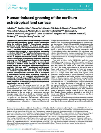
NATURE CLIMATE CHANGE DOI: 10.1038/NCLIMATE3056LETTERSa2.52.0Scaling factors1.51.00.50.0 0.5bLAI trend (m2 m 2 per 30 yr)0.40.30.20.10.0 ti31.00.80.60.40.20.0ti1RCTcFigure 4 Results from optimal D&A for 1982–2011 time series of LAIanomalies. a–c, The D&A analysis was performed over land of the NEL onensemble-mean 1982–2011 time series of LAI anomalies. Response patternswere derived from CMIP5 simulations accounting for both anthropogenicand natural forcings (ALL, in red), or greenhouse gas forcings only (GHG, ingreen), in a one-signal detection analysis. The observational average ofLAI3g and GEOLAND2 was used as reference in the analysis. Scalingfactors (β–see text) best estimates and their 90% confidence intervals (a),attributable trends over the 30-year-long time series (b) and p-value of theresidual consistency test (RCT) (c) are shown. Results were obtained froma total least square (TLS) analysis using the multi-model mean or selectedindividual model responses. ‘Multi1’ and ‘Multi3’ refer to two differentCMIP5 ensemble means (see text). Observational uncertainty wasassessed using individual satellite-derived observations (LAI3g orGEOLAND2) regressed onto the Multi1 response pattern.increased trends in vegetation indices1–5 , aboveground vegetationbiomass6,7 , and terrestrial carbon fluxes22 during the satellite era.Our analysis goes beyond previous studies by using D&A methodsto establish that the trend of strengthened northern vegetationgreening is clearly distinguishable from both IV and the responseto natural forcings alone. It can be rigorously attributed, withhigh statistical confidence, to anthropogenic forcings, particularlyto rising atmospheric concentrations of greenhouse gases. As anattempt to decipher which mechanisms are behind those trends, wefurther analysed the contribution of nitrogen deposition, LULCC,CO2 fertilization and GHG-induced climate change to the NELvegetation growth. This provides potential leads to understanding4the geographic structure of the vegetation response to selectedanthropogenic forcing agents.An accurate quantification of the responses to individual humanand natural drivers, however, needs more research efforts, owing touncertainties associated with the ESMs, weaknesses of the CMIP5experimental design, and limitations in the observations. Relativeto the observations, the simulations with ALL and GHG forcingsillustrated relatively weaker interannual variability of vegetationgrowth (Fig. 2 and Supplementary Figs 2 and 3). This discrepancymay arise from structural errors of the land component in the ESMs(for example, weak or no representation of vegetation mortality,disturbance and successional dynamics)23–25 . Because spatial andtemporal patterns of vegetation growth are tightly coupled withprecipitation variability4,17,18 , the underestimation could also arisefrom the reported underestimation of interannual precipitationvariability in CMIP models over Northern Hemisphere land26,27 .Multi-model ensemble means can have persistent biases, suchas overprediction of growing season length due to advancedspring growth and delayed autumn senescence in NorthernHemisphere temperate ecosystems17,28 . If such a phenological biaswere changing steadily over time, it could influence estimation ofLAI trends reported here. We mitigate against this type of bias bycomparing our results for different seasonal periods. Because ourresults are consistent for different definitions of growing season(Supplementary Figs 1–4 and 6), early and late season model biases,to the extent they are present in our multi-model data set, seemto be stationary in time. Understanding and ranking the multiplereasons for deficiencies in CMIP5 simulations, however, remainextremely difficult, given the lack of global LAI simulations withland surface models driven by common observed environmentalforcings. Such an obstacle should be overcome in the next phase ofCMIP, which will include an international intercomparison of theland surface components from the participating ESMs29 . Long-termremote-sensing data are often contaminated by clouds and snowcover, and are impacted by the change of satellites30 . For example,the LAI3g data set was probably influenced in 1991 by the eruptionof Mount Pinatubo and subsequent loss of orbit by NOAA 11,seen particularly in the world’s forests12 ; the merging of reflectanceinformation from different satellites during the pre- and post-2000periods for both LAI3g and GEOLAND2 products has the potentialto cause inhomogeneity in the data12,13 . These observational uncertainties, which are not considered here, might artificially increasethe observed interannual variability. Our sensitivity tests, however,show that our key findings are robust to these issues, and the fingerprint patterns assessed by the ALL and GHG ensembles can still beidentified quantitatively in the relatively short instrumental record.Given the strong evidence provided here of historical humaninduced greening in the northern extratropics, society shouldconsider both intended and unintended consequences of itsinteractions with terrestrial ecosystems and the climate system.MethodsMethods and any associated references are available in the onlineversion of the paper.Received 13 August 2015; accepted 16 May 2016;published online 27 June 2016References1. Myneni, R. B., Keeling, C., Tucker, C., Asrar, G. & Nemani, R. Increasedplant growth in the northern high latitudes from 1981 to 1991. Nature 386,698–702 (1997).2. Zhou, L. et al. Variations in northern vegetation activity inferred from satellitedata of vegetation index during 1981 to 1999. J. Geophys. Res. 106,20069–20083 (2001).3. Lucht, W. et al. Climatic control of the high-latitude vegetation greening trendand Pinatubo effect. Science 296, 1687–1689 (2002).NATURE CLIMATE CHANGE ADVANCE ONLINE PUBLICATION www.nature.com/natureclimatechange 2016 Macmillan Publishers Limited. All rights reserved
NATURE CLIMATE CHANGE DOI: 10.1038/NCLIMATE3056LETTERS4. Mao, J. et al. Global latitudinal-asymmetric vegetation growth trends and theirdriving mechanisms: 1982–2009. Remote Sens. 5, 1484–1497 (2013).5. Buitenwerf, R., Rose, L. & Higgins, S. I. Three decades of multi-dimensionalchange in global leaf phenology. Nature Clim. Change 5, 364–368 (2015).6. Pan, Y. et al. A large and persistent carbon sink in the world’s forests. Science333, 988–993 (2011).7. Liu, Y. Y. et al. Recent reversal in loss of global terrestrial biomass. Nature Clim.Change 5, 470–474 (2015).8. Ukkola, A. M. et al. Reduced streamflow in water-stressed climates consistentwith CO2 effects on vegetation. Nature Clim. Change 6, 75–78 (2015).9. Hegerl, G. C. et al. in Climate Change 2007: The Physical Science Basis (edsSolomon, S. et al.) 667–732 (IPCC, Cambridge Univ. Press, 2007).10. Bindoff, N. L. et al. in Climate Change 2013: The Physical Science Basis (edsStocker, T. F. et al.) 867–931 (IPCC, Cambridge Univ. Press, 2013).11. Cramer, W. et al. in Climate Change 2014: Impacts, Adaptation, andVulnerability (eds Field, C. B. et al.) 979–1037 (IPCC, CambridgeUniv. Press, 2014).12. Zhu, Z. et al. Global data sets of vegetation leaf area index (LAI) 3g and fractionof photosynthetically active radiation (FPAR) 3g derived from global inventorymodeling and mapping studies (GIMMS) normalized difference vegetationindex (NDVI3g) for the period 1981 to 2011. Remote Sens. 5, 927–948 (2013).13. Baret, F. et al. GEOV1: LAI and FAPAR essential climate variables andFCOVER global time series capitalizing over existing products. Part 1:Principles of development and production. Remote Sens. Environ. 137,299–309 (2013).14. Allen, M. & Stott, P. Estimating signal amplitudes in optimal fingerprinting,part I: theory. Clim. Dynam. 21, 477–491 (2003).15. Ribes, A., Planton, S. & Terray, L. Application of regularised optimalfingerprinting to attribution. part I: method, properties and idealised analysis.Clim. Dynam. 41, 2817–2836 (2013).16. Lamarque, J. F. et al. Multi-model mean nitrogen and sulfur deposition fromthe Atmospheric Chemistry and Climate Model Intercomparison Project(ACCMIP): evaluation of historical and projected future changes. Atmos.Chem. Phys. 13, 7997–8018 (2013).17. Anav, A. et al. Evaluation of land surface models in reproducing satellitederived leaf area index over the high-latitude northern hemisphere. part II:Earth system models. Remote Sens. 5, 3637–3661 (2013).18. Mahowald, N. et al. Projections of leaf area index in Earth system models.Earth Syst. Dynam. 7, 211–229 (2016).19. Menzel, A. et al. European phenological response to climate change matchesthe warming pattern. Glob. Change Biol. 12, 1969–1976 (2006).20. Zeng, F., Collatz, G., Pinzon, J. & Ivanoff, A. Evaluating and quantifying theclimate-driven interannual variability in Global Inventory Modeling andMapping Studies (GIMMS) Normalized Difference Vegetation Index(NDVI3g) at global scales. Remote Sens. 5, 3918–3950 (2013).21. Piao, S. et al. Evidence for a weakening relationship between interannualtemperature variability and northern vegetation activity. Nature Commun. 5,5018 (2014).22. Anav, A. et al. Spatio-temporal patterns of terrestrial gross primary production:a review. Rev. Geophys. 53, 785–818 (2015).23. McDowell, N. G. et al. Multi-scale predictions of massive conifer mortality dueto chronic temperature rise. Nature Clim. Change 6, 295–300 (2016).24. Di Vittorio, A. V. et al. From land use to land cover: restoring the afforestationsignal in a coupled integrated assessment–Earth system model and theimplications for CMIP5 RCP simulations. Biogeosciences 11, 6435–6450 (2014).25. Kunstler, G. et al. Plant functional traits have globally consistent effects oncompetition. Nature 529, 204–207 (2016).26. Zhang, X. et al. Detection of human influence on twentieth-centuryprecipitation trends. Nature 448, 461–465 (2007).27. Wu, P., Christidis, N. & Stott, P. Anthropogenic impact on Earth’s hydrologicalcycle. Nature Clim. Change 3, 807–810 (2013).28. Keenan, T. F. et al. Net carbon uptake has increased through warminginduced changes in temperate forest phenology. Nature Clim. Change 4,598–604 (2014).29. Eyring, V. et al. Overview of the Coupled Model Intercomparison ProjectPhase 6 (CMIP6) experimental design and organization. Geosci. Model. Dev.Discuss. 8, 10539–10583 (2015).30. Pinzon, J. E. & Tucker, C. J. A non-stationary 1981–2012 AVHRR NDVI3g timeseries. Remote Sens. 6, 6929–6960 (2014).AcknowledgementsThis work is supported by the Biogeochemistry-Climate Feedbacks Scientific Focus Areaproject funded through the Regional and Global Climate Modeling Program, and theTerrestrial Ecosystem Science Scientific Focus Area project funded through theTerrestrial Ecosystem Science Program, with additional support from the AcceleratedClimate Modeling for Energy project, in the Climate and Environmental SciencesDivision (CESD) of the Biological and Environmental Research (BER) Program in the USDepartment of Energy Office of Science. Oak Ridge National Laboratory is managed byUT-BATTELLE for DOE under contract DE-AC05-00OR22725. This work is supportedin part by the Fondation STAE, via the project Chavana. R.S. thanks the H2020 projectCRESCENDO ‘Coordinated Research in Earth Systems and Climate: Experiments,kNowledge, Dissemination and Outreach’, which received funding from the EuropeanUnion’s Horizon 2020 research and innovation programme under grant agreementno. 641816. R.B.M. is supported by NASA Earth Science Division through MODIS andVIIRS grants. B.W. is supported by the National Basic Research Program of China (Grantno. 2014CB441302). P.C. thanks the ERC SyG project IMBALANCE-P Effects ofphosphorus limitations on Life, Earth system and Society Grant agreement no. 610028.Author contributionsJ.M. conceived the study. J.M., A.R., B.Y., X.S., P.E.T. and R.S. performed diagnostics andwrote the text, with comments and edits from all authors.Additional informationSupplementary information is available in the online version of the paper. Reprints andpermissions information is available online at www.nature.com/reprints.Correspondence and requests for materials should be addressed to J.M.Competing financial interestsThe authors declare no competing financial interests.NATURE CLIMATE CHANGE ADVANCE ONLINE PUBLICATION www.nature.com/natureclimatechange 2016 Macmillan Publishers Limited. All rights reserved5
LETTERSNATURE CLIMATE CHANGE DOI: 10.1038/NCLIMATE3056Methodsforcing under scrutiny)32 are derived by multiplying the model-simulated trendand the estimated scaling factor β̂. Similarly, upper and lower bounds ofattributable trends are derived from the corresponding upper and lower bounds ofβ. We applied these statistical methods to the NEL average of three-year-mean LAI,as shown in Fig. 2. Natural internal variability is evaluated from unforced controlsimulations from several CMIP5 climate models, and expected response patternsare also taken from CMIP5 models (Supplementary Table 1).Detection and attribution. Two distinct statistical approaches were used to detectand attribute the LAI changes in this study. The simple comparison of observed andsimulated LAI trends (Fig. 3) is based on a simple T -test, which is further discussedin Supplementary Information 3. Then a more conventional D&A analysis is basedon an optimal regression technique in which observations Y are regressed onto theexpected response to historical forcing changes X (that is, Y X β ε, where εdenotes IV)14,15,31 . The scaling fact
The largest positive increase is observed in western Europe and eastern North America for both LAI products, . University of Texas, Austin, Texas 78712-1692, USA. 4Laboratoire des Sciences du Climat et de l . Institute of Atmospheric Physics, Beijing 100029, China. 13Center for Earth System Science, Tsinghua University, Beijing 100084 .