Transcription
119Part 2 / Basic Tools of Research: Sampling, Measurement, Distributions, and Descriptive StatisticsChapter 9Distributions: Population, Sampleand Sampling DistributionsIn the three preceding chapters we covered the three major steps in gathering and describingdistributions of data. We described procedures for drawing samples from the populations wewish to observe; for specifying indicators that measure the amount of the concepts contained inthe sample observations; and, in the last chapter, ways to describe a set of data, or a distribution.In this chapter we will expand the idea of a distribution, and discuss different types of distributions and how they are related to one another. Let us begin with a more formal definition of theterm “distribution”:A distribution is a statement of the frequency with which units of analysis (or cases) are assigned to the various classes or categories that make up a variable.To refresh your memory, a variable can consist of a number of classes or categories. The variable “Gender”, for instance, usually consists of two classes: Male and Female; “Marital Communication Satisfaction” might consist of the “satisfied”, “neutral”, and “dissatisfied” categories, and“Time Spent Viewing TV” could have any number of classes, such as 25 minutes, 37 minutes, and anumber of other values. The definition of a distribution simply states that a distribution tells us howmany cases or observations were seen in each class or category.For instance, a sample of 100 college students can be distributed in two classes which make upthe variable “Ownership of a CD Player”. Every observation will fall either in the “owner” or “nonowner” class. In our example, we might observe 27 students who “own a CD player” and a remaining 73 students who “do not own” a CD player. These two statements describe the distribution.Chapter 9: Distributions: Population, Sample and Sampling Distributions
120Part 2 / Basic Tools of Research: Sampling, Measurement, Distributions, and Descriptive StatisticsThere are three different types of distributions that we will use in our basic task of observationand statistical generalization. These are the population distribution, which represents the distribution of all units (many or most of which will remain unobserved during our research); the sampledistribution, which is the distribution of the observations that we actually make, after drawing asample from the population; and the sampling distribution, which is a description of the accuracywith which we can make statistical generalization, using descriptive statistics computed from theobservations we make within our sample.Population DistributionWe’ve already defined a population as consisting of all the units of analysis for our particularstudy. A population distribution is made up of all the classes or values of variables which we wouldobserve if we were to conduct a census of all members of the population. For instance, if we wish todetermine whether voters “Approve” or “Disapprove” of a particular candidate for president, thenall individuals who are eligible voters constitute the population for this variable. If we were to askevery eligible voter his or her voting intention, the resulting two-class distribution would be a population distribution. Similarly, if we wish to determine the number of column inches of coverage ofFortune 500 companies in the Wall Street Journal, then the population consists of the top 500 companies in the US as determined by the editors of Fortune magazine. The population distribution isthe frequency with which each value of column inches occurs for these 500 observations. Here is aformal definition of a population distribution:A population distribution is a statement of the frequency with which the units of analysis or cases thattogether make up a population are observed or are expected to be observed in the various classes or categories that make up a variable.Note the emphasized phrase in this definition. The frequency with which units of analysis areobserved in the various classes of the variable is not always known in a population distribution.Only if we conduct a census and measure every unit of analysis on some particular characteristic(that is, actually observe the value of a variable in every member of the population) will we be ableto directly describe the frequencies of this characteristic in each class. In the majority of cases wewill not be in a position to conduct a census. In these cases we will have to be satisfied with drawinga representative sample from the population. Observing the frequency with which cases fall in thevarious classes or categories in the sample will then allow us to formulate expectations about howmany cases would be observed in the same classes in the population.For example, if we find in a randomly selected (and thus representative) sample of 100 collegeundergraduates that 27 students own CD players, we would expect, in the absence of any information to the contrary, that 27% of the whole population of college undergraduates would also have aCD player. The implications of making such estimates will be detailed in following chapters.The distribution that results from canvassing an entire population can be described by usingthe types of descriptive indicators discussed in the previous chapter. Measures of central tendencyand dispersion can be computed to characterize the entire population distribution.When such measures like the mean, median, mode, variance and standard deviation of a population distribution are computed, they are referred to as parameters. A parameter can be simplydefined as a summary characteristic of a population distribution. For instance, if we refer to the factthat in the population of humans the proportion of females is .52 (that is, of all the people in thepopulation, 52% are female) then we are referring to a parameter. Similarly, we might consult atelevision programming archive and compute the number of hours per week of news and publicaffairs programming presented by the networks for each week from 1948 to the present. The meanand standard deviation of this data are population parameters.You probably are already aware that population parameters are rarely known in communication research. In these instances, when we do not know population parameters we must try to obtain the best possible estimate of a parameter by using statistics obtained from one or more samplesdrawn from that population. This leads us to the second kind of distribution, the sample distribution.Chapter 9: Distributions: Population, Sample and Sampling Distributions
121Part 2 / Basic Tools of Research: Sampling, Measurement, Distributions, and Descriptive StatisticsSample DistributionAs was discussed in Chapter 5, we are only interested in samples which are representative ofthe populations from which they have been drawn, so that we can make valid statistical generalizations. This means that we will restrict our discussion to randomly selected samples. These randomprobability samples were defined in Chapter 6 as samples drawn in such a way that each unit ofanalysis in the population has an equal chance of being selected for the sample.A sample is simply a subset of all the units of analysis which make up the population. Forinstance, a group of voters who “Approve” or “Disapprove” of a particular presidential candidateconstitute a small subset of all those who are eligible voters (the population). If we wanted to determine the actual number of column inches of coverage given to Fortune 500 companies in the WSJ wecould draw a random sample of 50 of these companies. Below is a definition of a sample distribution:A sample distribution is a statement of the frequency with which the units of analysis or cases thattogether make up a sample are actually observed in the various classes or categories that make up avariable.If we think of the population distribution as representing the “total information” which wecan get from measuring a variable, then the sample distribution represents an estimate of this information. This returns us to the issue outlined in Chapter 5: how to generalize from a subset of observations to the total population of observations.We’ll use the extended example from Chapter 5 to illustrate some important features of sampledistributions and their relationship to a population distribution. In that example, we assumed thatwe had a population which consisted of only five units of analysis: five mothers of school-agedchildren, each of whom had differing numbers of conversations about schoolwork with her child inthe past week.The population parameters are presented in Table 9-1, along with the simple data array fromwhich they were derived. Every descriptive measure value shown there is a parameter, as it is computed from information obtained from the entire population.Chapter 9: Distributions: Population, Sample and Sampling Distributions
122Part 2 / Basic Tools of Research: Sampling, Measurement, Distributions, and Descriptive StatisticsChapter 9: Distributions: Population, Sample and Sampling Distributions
123Part 2 / Basic Tools of Research: Sampling, Measurement, Distributions, and Descriptive StatisticsBut we know that a sample will contain a certain amount of sampling error, as we saw inChapter 5. For a refresher, see Table 5-6 in that chapter for a listing of all the samples and theirmeans that would be obtained if we took samples of N 3 out of this population. Table 9-2 showsjust three of the 125 different sample distributions that can be obtained when we do just this.Since the observed values in the three samples are not identical, the means, variances, andstandard deviations are different among the samples, as well. These numbers are not identical to thepopulation parameters shown in Table 9-1. They are only estimates of the population values. Therefore we need some way to distinguish between these estimated values and the actual descriptivevalues of the population.We will do this by referring to descriptive values computed from population data as parameters, as we did above. We’ll now begin to use the term statistics, to refer specifically to descriptiveindicators computed from sample data. The meaning of the term statistic is parallel to the meaningof the term parameter: they both characterize distributions. The distinction between the two lies inthe type of distribution they refer to. For sample A, for instance, the three observations are 5, 6 and7; the statistic mean equals 6.00 and the statistic variance is determined to be .66. However, theparameter mean and parameter variance are 7.00 and 2.00, respectively. In order to differentiatebetween sample and population values, we will adopt different symbols for each as shown in Table9-3.One important characteristic of statistics is that their values are always known. That is, if wedraw a sample we will always be able to calculate statistics which describe the sample distribution.In contrast, parameters may or may not be known, depending on whether we have census information about the population.One interesting exercise is to contrast the statistics computed from a number of sample distributions with the parameters from the corresponding population distribution. If we look at the threesamples shown in Table 9-2, we observe that the values for the mean, the variance, and the standarddeviation in each of the samples are different. The statistics take on a range of values, i.e., they arevariable, as is shown in Table 9-4.The difference between any population parameter value and the equivalent sample statisticindicates the error we make when we generalize from the information provided by a sample to theactual population values. This brings us to the third type of distribution.Chapter 9: Distributions: Population, Sample and Sampling Distributions
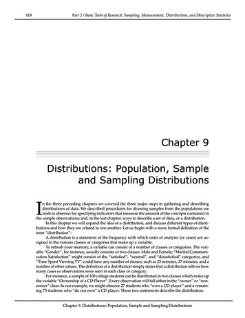
124Part 2 / Basic Tools of Research: Sampling, Measurement, Distributions, and Descriptive StatisticsSampling DistributionIf we draw a number of samples from the same population, then compute sample statistics foreach, we can construct a distribution consisting of the values of the sample statistics we’ve computed. This is a kind of “second-order” distribution. Whereas the population distribution and thesample distribution are made up of data values, the sampling distribution is made up of values ofstatistics computed from a number of sample distributions.Probably the easiest way to visualize how one arrives at a sampling distribution is by lookingat an example. We’ll use our running example of mothers’ communication with children in whichsamples of N 3 were selected. Figure 9-1 illustrates a model of how a sampling distribution isobtained.Figure 9-1 illustrates the population which consists of a set of scores (5, 6, 7, 8 and 9) whichdistribute around a parameter mean of 7.00. From this population we can draw a number of samples.Each sample consists of three scores which constitute a subset of the population. The sample scoresdistribute around some statistic mean for each sample. For sample A, for instance, the scores are 5,6 and 7 (the sample distribution for A) and the associated statistic mean is 6.00. For sample B thescores are 5, 8 and 8, and the statistic mean is 7.00. Each sample has a statistic mean.The statistics associated with the various samples can now be gathered into a distribution oftheir own. The distribution will consist of a set of values of a statistic, rather than a set of observedvalues. This leads to the definition for a sampling distribution:A sampling distribution is a statement of the frequency with which values of statistics areobserved or are expected to be observed when a number of random samples is drawn from a givenpopulation.It is extremely important that a clear distinction is kept between the concepts of sample distribution and of sampling distribution. A sample distribution refers to the set of scores or values thatwe obtain when we apply the operational definition to a subset of units chosen from the full population. Such a sample distribution can be characterized in terms of statistics such as the mean, variance, or any other statistic. A sampling distribution emerges when we sample repeatedly and recordChapter 9: Distributions: Population, Sample and Sampling Distributions
125Part 2 / Basic Tools of Research: Sampling, Measurement, Distributions, and Descriptive Statisticsthe statistics that we observe. After a number of samples have been drawn, and the statistics associated with each computed, we can construct a sampling distribution of these statistics.The sampling distributions resulting from taking all samples of N 2 as well as the one basedChapter 9: Distributions: Population, Sample and Sampling Distributions
126Part 2 / Basic Tools of Research: Sampling, Measurement, Distributions, and Descriptive Statisticstaking all samples of N 3 out of the population of mothers of school-age children are shown inTable 9-5.These sampling distributions are simply condensed versions of the distributions presentedearlier in Tables 5-1 and 56. In the first column we can see the various means that were observed. Thefrequency with which these means were observed is shown in the second column. The descriptivemeasures for this sampling distribution are computed next and they are presented below.The first such measure computed is a measure of central tendency, the mean of all the samplemeans. This is frequently referred to as the grand mean, and it is symbolized like this:From the values in the sampling distribution we can also compute measures of dispersion.Using the difference between any given statistic mean and the grand mean, we can compute thevariance and the standard deviation of the sampling distributions, as illustrated in columns 4, 5 and6 of Table 9-5. In the fourth column we determine the difference between a given mean and thegrand mean; in column five that difference is squared in order to overcome the “Zero-Sum Principle”, and in column six the squared deviation is multiplied by f to reflect the number of times thata given mean (and a given difference between a statistic mean and the grand mean, and the squaredvalue of this difference) was observed in the sampling distribution. As you see, the descriptivemeasures in a sampling distribution parallel those in population and sample distributions. To avoidChapter 9: Distributions: Population, Sample and Sampling Distributions
127Part 2 / Basic Tools of Research: Sampling, Measurement, Distributions, and Descriptive Statisticsthe confusion that may be caused by this similarity we will use a set of special terms for thesedescriptive measures. The variance of a sampling distribution will be referred to as sampling variance and the standard deviation of the sampling distribution will be called the standard error. Table9-6 provides a listing that allows for an ready comparison of the three main types of distributions,what the distributions consist of, and the labels of the most frequently used descriptive measures.Maintaining these different symbols and labels is important. Whenever we see, for instance, M 4.3, we know that 4.3 is the mean of a population, and not the mean of a sample or samplingdistribution. Furthermore, whenever the term sd is used we know that the measure refers to thevariability of scores from a sample; whenever the term std error is encountered we know that reference is being made to dispersion within a distribution of statistics.The Utility of a Sampling DistributionBy now it should be clear how a sampling distribution might be constructed. However, questions about the utility of doing so may remain. Why do we bother to construct sampling distributions, particularly sampling distributions of means? There are three reasons for constructing sampling distributions of means. In a nutshell, these sampling distributions give us insight into sampling error; they give insight into probability; and they allow us to test hypotheses.Sampling Distributions as Distributions of Sampling ErrorIn Chapter 5 we encountered the term sampling error when we discussed random sampling.When we draw random samples from a population there are no guarantees that the sample willindeed be exactly representative of the population. As seen earlier in this chapter it is quite possiblethat there will be differences between sample characteristics and population characteristics. In fact,sampling error can be defined as the discrepancy between the parameter of a population and thecorresponding statistic computed for a sample drawn randomly from that population.One way of looking at Table 9-5 is as an illustration of sampling error. It shows a listing of allthe sample statistic means that were computed when all possible samples of a given size were drawnfrom the population. Most of these different statistic means show a certain amount of discrepancywith the population mean; some means show larger discrepancies, others show smaller ones (seecolumn 4). The sampling distribution that result when we take all samples from a given populationis therefore also the distribution of the amounts of sampling error that we encountered as we drewthose samples.Sampling Error and the Standard ErrorWe know that sampling error is unavoidable, even when we sample randomly. However, letus assume for a moment that we could randomly sample without committing sampling error. Inthat case, for all the samples that we would draw from a population, there would be no discrepancybetween the statistic computed for each sample and the population parameter. Each sample meanwould be exactly equal to the population mean. Since all the entries in the sampling distributionwould be identical, the sampling distribution would have a mean equal to the population mean.The sampling variance and the standard error are measures of dispersion of a set of statistics aboutthe mean of the sampling distributio
Fortune 500 companies in the Wall Street Journal, then the population consists of the top 500 com-panies in the US as determined by the editors of Fortune magazine. The population distribution is the frequency with which each value of column inches occurs for these 500 observations.