Transcription
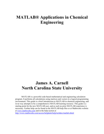
MATLAB Applications in ChemicalEngineeringJames A. CarnellNorth Carolina State UniversityMATLAB is a powerful code-based mathematical and engineering calculationprogram. It performs all calculations using matrices and vectors in a logical programmingenvironment. This guide is a brief introduction to MATLAB in chemical engineering, andin no way attempts to be a comprehensive MATLAB learning resource. This guide is astarting point for the new MATLAB user, and as such no prior MATLAB experience isnecessary. Further help can be found in the MATLAB help files or at Mathworks websiteat www.mathworks.com and in the help section chdoc/matlab.shtml
MATLAB Applications in Chemical EngineeringJames A. Carnell, August 2003Table of ContentsSection I: How MATLAB Works» Basic MATLAB: The Language» Mfiles (Function files)» Dealing with Functions The ‘plot’ function The ‘fzero’ function Solving linear equations in MATLAB The ‘fsolve’ functionSection II: Numerical and Symbolic Integration» Numerical Integration; Quadrature The Simpson’s Rule and Lobotto Quadrature» Symbolic Integration and DifferentiationSection III: Numerically Solving Differential Equations and Systems of DifferentialEquations» First order ode’s» Higher order ode’sAppendix» Glossary of Commands, Parts I, II and II» Line Markers
MATLAB Applications in Chemical EngineeringJames A. Carnell, August 2003Section I: How MATLAB worksMost MATLAB commands can be run from the command window (shown below,on the right hand side of the interface). MATLAB commands can also be entered into atext file labeled with the ‘.m’ extension. These files are known as ‘m-files’. Thesecommands can be broken down into scripts and programming. Scripts can be thought ofas commands that instruct MATLAB to execute a particular function or pre-madeprogram, and programming can be thought of as the raw code required to constructfunctions and programs within MATLAB. Generally, all programming must be containedwithin a file used by MATLAB (called an m-file), but script can be entered either in anm-file or directly into the command window. An image of the MATLAB interface isshown below.MATLAB contains many ready-made programs or functions that are convenientlyarranged into different toolboxes. When using MATLAB, these toolboxes and theirfunctions can be called upon and executed in any MATLAB script. In the above image,the toolbox selection or launch pad is shown (at the left hand side of the interface).Basic MATLAB: The languageMATLAB uses a language that is somewhat similar to that of Maple1. The scriptsor calling functions have a particular name and argument that must be entered into thefunction execution call. For example, to plot the sine function in MATLAB between 0and 6 using the fplot command, the following code can be entered directly into thecommand window, or into an m-file:1Maple is a registered trademark of Waterloo Maple, Inc.
MATLAB Applications in Chemical EngineeringJames A. Carnell, August 2003(One can define the function sin(x) in an m-file and replace the fplot command to befplot(‘filename’,[0,6]))Before going much further, an understanding of the structure of a MATLABsimulation or execution must be developed.M-filesM-files contain programming, scripts, equations or data that are called uponduring an execution. If the m-file is a function definition, then the most important part ofthis type of m-file is the first line. The first line must contain the function definition sothat MATLAB can find those m-files that are called upon. These types of m-files arecalled function m-files or function files. The code used to define the function file is asfollows:‘file name’ is simply the name of the m-file (the filename must be the same in thedefinition and the file-name), z is the dependant variable, and x and y are the independentvariables. (Of course, one can have less or more independent variables depending uponthe complexity of the problem and the equations involved.) The next few lines of script inthe m-file can define the function or functions and label any required variables. Thefollowing is an example of an m-file used to plot the natural logarithm2 function.To produce a plot of this function, the following code is entered into the commandwindow:This yields a plot of ln(x) between x 1 and x 5.2MATLAB uses ‘log’ as the natural logarithm function, and ‘log10’ as logarithm base ten.
MATLAB Applications in Chemical EngineeringJames A. Carnell, August 2003Using the ‘insert’ menu one can add a title, x and y axis titles, and if necessary a legend.One can also use commands nested within the fplot command to title the chart, add axistitles, or decide upon curve characteristics such as line color or marker.Dealing with functionsStandard functions such as the sine, cosine, logarithmic, exponential, and userdefined functions within MATLAB will now be covered. fplot has already beenintroduced; now plot, fzero and fsolve will be introducedThe ‘plot’ functionThe plot function produces a 2-D plot of a y-vector versus either its real index or aspecified x-vector. The plot function can be used for data, standard functions, or userdefined functions. Let’s look at a simple example of using plot to model data.Example 1.1The following reaction data has been obtained from a simple decay reaction:AÆBUse MATLAB to plot the concentration of component A in mol/L against the reactiontime, t, in minutes. Title the plot, label the axes, and obtain elementary statistics for thedata.
MATLAB Applications in Chemical EngineeringJames A. Carnell, August Liter)1008065554945424138SolutionFirst, the data must be entered into MATLAB as two vectors. The vectors x and yare defined in the command window, followed by the command to plot the data. Thefollowing graph is displayed:
MATLAB Applications in Chemical EngineeringJames A. Carnell, August 2003The ‘x’ row matrix (or vector*) has its display output suppressed using the ‘;’ at the endof the line.Syntax can be used to specify the title and labels, but an easier GUI (GraphicalUser Interface) based approach is to simply edit the figure. Select the ‘Edit Plot’ command found in the ‘Tools’ menu, or click thenorth-west facing arrow icon on the figure. Double click on the white-space in the graph. This enables the propertyeditor. Now the title and axes can be inserted under the ‘labels’ command. Now click directly on the line, and the line property editor will come up.Now the lines color, pattern, or the markers can be edited. The final curveis presented below:*A single row matrix or column matrix can represent vectors within MATLAB.
MATLAB Applications in Chemical EngineeringJames A. Carnell, August 2003Solution curve to example 1.1NOTE: These figures can be exported in .bmp or .jpg format so they can be made part of a document. Findthese under the ‘FileÆExport’ menu.To display simple statistics of the data, follow the path, ‘ToolsÆData Statistics’ and theminimum, maximum, mean, median, standard deviation, and range of x and y will bedisplayed. Within this box, each statistic can be added to the curve as a data point/line.To plot functions using plot, an m-file can be created defining the function, or thedefinition can be specified in the command window. This is done in a similar fashion asseen in ‘fplot’. The following code entered into the command window yields a plot of theexponential function between 0 and 10, at intervals of 1.
MATLAB Applications in Chemical EngineeringJames A. Carnell, August 2003There are many other 2-D plotting functions in Matlab, but fplot, plot and ezplot are themost useful. ‘ezplot’ is another way to quickly plot functions between specified or nonspecified (-2π x 2π) intervals. The syntax key for ezplot is shown below.This can be used to plot f(x) or f(x(t),y(t)).The ‘fzero’ functionThe fzero function is a convenient function used to find local zeros of a onevariable function. The general syntax that can be used for fzero (entered into thecommand window) isx fzero(‘function’,initial guess)Matlab will then return the solution or a NaN result. An NaN result is ‘not a number’ andrepresents a ‘no solution’ for the function. Below are a few examples relating to fzero.Example 1.2Find the zero of the function y(x) x2-1 using an m-file and fzero.SolutionCreate the m-file, ‘myfunction.m’function y myfunction(x)y x 2-1In the command window, use fzero to find the zero of the function ‘myfunction’x fzero(‘myfunction’,3)Matlab returns a few iterations and then produces the result ‘x 1’
MATLAB Applications in Chemical EngineeringJames A. Carnell, August 2003Example 1.3Find the zero of the function y(x) sin(x) closest to x 3 using the fzero commanddirectly in the command window. Do not use an m-file for this example.SolutionEnter into the command window x fzero(‘sin(x)’,3) Matlab returns avalue of 3.1416. This is the zero of sin(x) closest to our initial guess of 3.Solving linear equations in MatlabMatlab has the ability to easily solve linear equations directly on the commandwindow. The following example will demonstrate how to do this in Matlab.Example 1.4Solve the system of linear equations given below using Matlab.3.5u 2v 5 1.5u 2.8v 1.9 w 1 2.5v 3w 2SolutionEnter the following code directly into the clear Matlab command window. (If thewindow is not clear, enter the command ‘clear’ to clear the memory of any variables).The matrix ‘a’ contains the coefficients of u, v and w respectively. Each row in the matrix(there are three) corresponds to the coefficients of u, v and w in that order. Matrix ‘b’contains the solution to each row or equation, 5, -1 and 2. The matrix ‘x’ that is dividedout can be thought of as containing the values for u, v and w.The solutions to the equations are displayed as u, v and w as they are listed in the matrix.The command a\b′ performs reverse matrix division. The ′ command transposes matrix b,this is required to perform matrix division. It is a property of matrices. Essentially, the
MATLAB Applications in Chemical EngineeringJames A. Carnell, August 2003matrix is in the form Ax B, the command a\b′ can be thought of as ‘dividing out’ thevalues of x. (Alternatively, the command ‘b/a′’ will also yield the correct solution set.)The ‘fsolve’ functionThe ‘fsolve’ function will probably be the most useful function for simplechemical engineering problems. It is essentially a numeric solver, capable of solvingsystems of non-linear continuous equations.For the system of n continuous equations (f1--fn) with n unknown variables (x1-xn) given byf (1) f 1 ( x1 , x 2 , x3 ,., x n ) 0f (2) f 2 ( x1 , x 2 , x3 ,., x n ) 0f (3) f 3 ( x1 , x 2 , x3 ,., x n ) 0.f (n) f n ( x1 , x 2 , x3 ,., x n ) 0Matlab’s solver can be used to determine the unknown variables, x1 through xn. Thefollowing example will illustrate the use of the fsolve function.Example 1.5Solve the system of equations below using fsolve.2a b e a 02b a e b 0SolutionThe most efficient way to solve these types of systems is to create a function mfile that contains the equations.The equations are separated within the matrix ‘f’ using the semi-colon operator. Now the‘fsolve’ command must be used to solve the system.
MATLAB Applications in Chemical EngineeringJames A. Carnell, August 2003The solutions to the system are a 0.5671 and b 0.5671 . Using the ‘fsolve’ command,much more complicated systems can be easily solved in Matlab. NOTE: ‘optimset’ isused to change the default solver in Matlab to the optimization toolbox solver (fsolve, 2.0onwards)Section II: Numerical and Symbolic integrationNumerical Integration-QuadratureMATLAB can perform in-depth numerical integrations or quadrature effortlesslyand accurately. The first part of this section will look at some of the simple methods ofnumerical integration within MATLAB.The Simpson’s Rule and Lobotto QuadratureIn MATLAB, the functions ‘quad’ or in more recent versions, ‘quadl’ performnumerical integration based on the Simpson’s rule and the adaptive Lobatto quadraturerespectively. The syntax for the Simpson’s based approximation and the Lobottoquadrature are the same. The difference is in each function’s name. The syntax below isfor the Lobotto quadrature (quadl), and it is the same for the Simpson’s quadrature(quad).q quadl(fun,a,b)q quadl(fun,a,b,tol)q quadl(fun,a,b,tol,trace)q quadl(fun,a,b,tol,trace,p1,p2,.)[q,fcnt] quadl(fun,a,b,.)The functions can be defined in function m-files or as inline functions (those functionsentered directly into the command). MATLAB also has a function called ‘trapz’ whichenables numerical integration using the trapezoid rule. More information about ‘trapz’can be found in the MATLAB help files.Symbolic Integration and differentiationMatlab has the ability to perform symbolic integration and differentiation thanksto the Maple engine located in the symbolic toolbox. Matlab can solve differentialequations symbolically, providing general or unique solutions. First, let’s look atsymbolic integration and differentiation.Using the ‘diff’ command, symbolic differentiation of a function can be achieved,and analogously, using the ‘int’ command symbolic integration of a function can beachieved. Example 2.1 demonstrates use of the ‘int’ and ‘diff’ commands.Example 2.1Integrate ax2 bx, with respect to x, (where a and b are constant) and thendifferentiate the solution obtained with respect to x to regain the initial function.SolutionTo begin with, the symbolic variables within the expression must be definedwithin MATLAB as symbolic variables. This is done using the syms command. In the
MATLAB Applications in Chemical EngineeringJames A. Carnell, August 2003expression, a, b, and x are the symbolic variables that must be defined. The followingcode is used directly at the command prompt to obtain the solution:The syms command is used to define a, b and x as variables for symbolic purposes. Theexpression is differentiated to obtain the solution 2ax b, which upon integration withrespect to x yields ax2 bx as expected.MATLAB can solve ordinary differential equations symbolically with or withoutboundary conditions or initial value parameters. The ‘dsolve’ command is used for thispurpose. Within dsolve, the letter ‘Dij’ is used to indicate a derivative, where i is theorder of differentiation, and j is the dependent variable. ‘D’ implicitly specifies first orderderivative, ‘D2’ signifies a second order derivative and so on. The letter t is the defaultd2yindependent variable for dsolve. So D2y is analogous to 2 . The following exampledtillustrates the use of dsolve.Example 2.2Solve the oded2ydy 6y , where y(x) using dsolvedxdxSolutionWhere C1 and C2 are constants of integration.The next example shows how to solve an initial value problem for a second order ode.
MATLAB Applications in Chemical EngineeringJames A. Carnell, August 2003Example 2.3dmd 2mSolve the ode m 0 , m(0) 2 and(0) 3 , where m(x).2dxdxSolutionWithin dsolve, m(0) 2 and Dm(0) 3 define the initial conditions of the ode.In the assignment of the initial conditions, labeled variables could have been insertedrather than numeric values. For example, if the initial conditions for example 2.3 weredm(0) b , then the command chainm(0) a anddxcould have been used to yield the solution.Section III: Numerically Solving Differential Equations and Systems of DifferentialEquationsFirst order ode’sOne of the best engineering uses of MATLAB is its application to the numericsolution of ordinary differential equations (ode’s). MATLAB has multiple different odesolvers that allow ode’s to be solved accurately and efficiently depending on the stiffnessof the ode. Stiffness is the relative change in the solution of a differential equation. A stiffdifferential equation is one that the solution changes greatly when close to the point ofintegration, but need not change significantly over the duration of the integration. For thistype of solution, a numerical method that takes small integration intervals rather thanlarge intervals would be required. Stiffness and solver selection are mainly a matter ofefficiency. In solving ode’s, selecting a solver that takes the largest step, yet stillmaintains an accurate solution is the key to increased efficiency.There are different ways to set up and execute the ode solvers, but for this guide, asystem that uses multiple m-files per each ode solution will be employed. The main twom-files that are needed are a run file and a function file. For the solution of ode’s inMATLAB all ode’s must be defined in a function m-file. When entered into the functiondyfile, the ode’s must have the first order form f ( y, x) . The function file must containdxi)The function definition e.g.,where t is theindependent variable and m is the dependent variable of first order
MATLAB Applications in Chemical EngineeringJames A. Carnell, August 2003ii)If global variables are used, the global command must be inserted after thefunction definitioniii)The ode or ode’s in the form described above e.g.The filename, variables (m and t) and dmdt are arbitrary. ‘dmdt’ is also arbitrary and canequivalently be called ‘A’ or any other non-reserved name. One stipulation that exists isthat the definition within the ‘function dmdt file name(t,m)’ MUST be the same as thatdefined when the ode’s are listed. For example, the following function m-file is incorrectfunction dmdt myfile(t,m)A 4*mBut, the following function file is correct:function dmdt myfile(t,m)dmdt 4*m(It may appear that from this MATLAB is unable to solve any more than a first orderode, but all ode’s of second order or higher can be written in the form of multiple ode’s,each of first order. This will be covered once an introduction using first order ode’s hasbeen accomplished).Once a suitable function file has been created, a run-file or executable file iscreated that is used to solve the ode or ode’s that are within the function file. The run filemust contain the following items:i)If global variables are used, the global command must be inserted at thispoint.ii)Depending on how the tspan, the integration interval, is defined, the lowerand upper limits can be defined here. E.g., where t0 and tfare predefined vectors for the integration limits. Forward or reverseintegration can be used; t0 does not have to be less than tf in the case ofreverse integrationiii)The initial conditions must be defined as vectors or single directionmatrices.iv)The ode solver must then be called. The following is the syntax for thesolver, and ode45 is the solver that will be used. It is a good place to startas a general solver:v)The solution can now be plotted using the ‘plot’ command and thenformatted either using the GUI interface or by the commands ‘legend’,‘xlabel’, ‘ylabel’, ‘title’ and ‘axis’. E.g.st,where n denotes the 1 dependent variable, then second and so on.The following example demonstrates the setup and execution for the solution of a set ofdifferential equations.
MATLAB Applications in Chemical EngineeringJames A. Carnell, August 2003Example 3.1A fluid of constant density starts to flow into an empty and infinitely large tank at8 L/s. A valve regulates the outlet flow to a constant 4L/s. Derive and solve thedifferential equation describing this process over a 100 second interval.SolutionThe accumulation is described as input – output, so the ode describing the processd ( ρV )dvbecomes (8 4) ρ . Since density is constant, then 8 4 4 in liters perdtdtsecond. The initial condition is that at time t 0, the volume inside the tank 0. Thefollowing function file ‘ex31’ is used to set up the ode solver.The file ex31run is used to execute the solver. The code for this file is overleaf.The plot produced is
MATLAB Applications in Chemical EngineeringJames A. Carnell, August 2003As expected, a constant volume increase of 4L/s is described by the curve.Systems of ode’s can also be easily solved in MATLAB using the same setup asdescribed for a single ode. Example 3.2 demonstrated how to solve a system ofsimultaneous ode’s. In example 3.2 the ‘global’ command is used to define certainvariables as ‘shared’ or ‘in common’ between the run file and the function file. Globalvariables are not necessary, but they are convenient. Using the ‘global’ commandvariables can be defined once in the run file and the global command will link them to thefunction file. If used, the global command must not contain the independent or dependentvariables.Example 3.2The following set of differential equations describes the change in concentrationthree species in a tank. The reactions AÆBÆC occur within the tank. The constants k1,and k2 describe the reaction rate for AÆB and BÆC respectively. The following ode’sare obtained:dCa k1CadtdCb k1Ca k 2CbdtdCc k 2Cbdt
MATLAB Applications in Chemical EngineeringJames A. Carnell, August 2003Where k1 1 hr-1 and k2 2 hr-1 and at time t 0, Ca 5mol and Cb Cc 0mol. Solve thesystem of equations and plot the change in concentration of each species over time.Select an appropriate time interval for the integration.SolutionThe following function file and run file are created to obtain the solution:Ca, Cb and Cc must be defined within the same matrix, and so by calling Ca c(1), Cb c(2)and Cc as c(3), they are listed as common to matrix c.Notice that the constants k1 and k2 are defined (only once) in the run file, and using the‘global’ command they are linked to the function file. The following curve is producedupon execution. In the ‘plot’ command, the and * change the line markers so that theycan be easily distinguished using a non-color printer. The appendix contains a list ofavailable markers for plotting.
MATLAB Applications in Chemical EngineeringJames A. Carnell, August 2003Higher order ode’sTo be able to solve higher order ode’s in MATLAB, they must be written in termsof a system of first order ordinary differential equations. An ordinary differentialequation can be written in the formdny f ( x, y, y ′, y ′′, y ′′′,., y n 1 )ndxand can also be written as a system of first order differential equations such thaty1 y, y 2 y ′, y 3 y ′′,. y n y n 1 .From here, the system can then be represented as an arrangement such thaty1′ y 2 , y 2′ y 3 ,. y ′n 1 y n , where y'n f(x,y1,y2,.yn).Example 3.3 demonstrates this technique.Example 3.3Solve the following differential equation by converting it to a system of first orderdifferential equations, then using a numeric solver to solve the system. Plot the results.
MATLAB Applications in Chemical EngineeringJames A. Carnell, August 2003Y ′′ Y ′ Y 0 , Y(0) 1 and Y'(0) 0To convert this 2nd order ode to a system of 1st order ode’s, the following assignment ismade:Y y1 y (1) and Y ′ y 2 y (2) ,then the ode can be written as the first-order system:Y y (1)dY Y ′ y (2)dtd 2Y Y ′′ ( y (2) y (1))dt 2The function file containing this system can now be created and solved. The function fileand run file are shown below:The variable dmdt is a ‘dummy’ variable that is used to describe the system as a whole,The following curve is produced
MATLAB Applications in Chemical EngineeringJames A. Carnell, August 2003The appendices of this guide are designed to be used as ‘cheat-sheets’ to aid in usingMATLAB without simply manipulating the examples herein. Successful use ofMATLAB comes from understanding how and why it works the way it does. MATLABcan be used for almost anything that requires calculation and so frequent use for simpletasks will aid in the competency of the package.
MATLAB Applications in Chemical EngineeringJames A. Carnell, August 2003AppendixMATLAB Glossary of commands (Part 1) Matrix commands (A is an arbitrary matrix)» sum(A)Æ Summation of the rows of matrix A» A’Æ Transposes matrix A» diag(A)Æ Takes the diagonal values of square matrix A» fliplr(A) Æ Flips matrix A from left to right» 1:n:10Æ Fills sequence of numbers, 1 to 10 with spacing n (if n isnot stipulated, then MATLAB will assume n 1) Command Window» clear Æ Clears memory of variables» clcÆ Clears command window (clf will clear the figure window)» Æ Wraps text or code if required, (followed by return or enter)» up arrowÆ Recalls last line» ;Æ Output suppression ( eg. Does not SHOW output)» iskeyword Æ Displays reserved MATLAB keywords Functions and other commands» plot(independent, dependent) ÆA graphing command.Independent variables must be defined before using the plot command.» fplot(‘function’,[xmin, xmax, ymin, ymax])ÆGraphs afunction either from an m-file or direct command, the function entered canbe a file-name linking to an m-file or it can the the function itself e.g.‘sin(x)’» ezplot(‘function’,[xmin, xmax, ymin, ymax])ÆAsabove» fsolve(‘m-file-name’,initial guess,options) Æ Solvesnon-linear continuous systems of equations. Initial guess usually in theform of a matrix, predefined. Usual option is ‘optimset(‘fsolve’)’» x fzero(‘function’,initial guess)ÆNumerically finds thezero of the function close to the initial guess. The function can be in an mfile or a direct command (similar to fplot). The initial guess can be entereddirectly, or in the form of a predefined vector. The in-line function mustbe in terms of x only. It cannot contain any predefined constants.» m input(‘m ’)ÆRequests that an input variable be entered intoMATLAB, which is then saved as ‘m’ or any other arbitrary name. Usedin m-files» display(‘text to be displayed’) ÆDisplays ‘text to bedisplayed’ in a matlab execution. Used in m-filesIn all of the above function definitions, the ’notation must be included in the MATLABcommand execution. For example, the fzero command to find the zero of x3, one woulduse the notation: x fzero(‘x 3’,1), where 1 is the initial guess.
MATLAB Applications in Chemical EngineeringJames A. Carnell, August 2003MATLAB glossary of commands (Part II)Symbolic integration and differentiation» syms v1 v2 Æ Declares variable v1 and v2 as symbolic variables,used for symbolic integration and differentiation» int(exp1,independent)Æ Performs symbolic integration of exp1with respect to independent variable ‘independent’» diff((exp1,independent) Æ Performs symbolic differentiationof exp1 with respect to independent variable ‘independent’» dsolve(‘ode1,ode2,oden’, ‘bc1,bc2,bcn’, ‘IV’)ÆPerforms symbolic ode solving, where ode1, ode2 and oden are systemsof ode’s and bc1, bc2 and bcn are their respective boundary conditions. IVis the common independent variable. The default IV is t, so if no IV isspecified, then t is assumed to be the independent variable. To indicate aderivative the capital letter ‘D’ is used, followed by the order then thed2ydependent variable. So D2y represents. For non-boundaryd (IV ) 2condition problems, the ‘bc1,bc2,bc3’ term can be negated and thesolution will be returned containing integration constants.» simplify(A) Æ Simplifies expression A
MATLAB Applications in Chemical EngineeringJames A. Carnell, August 2003MATLAB glossary of commands (Part III)The sequence of this sheet hints towards the correct sequence for solving odes in matlab1. The different ODE solvers:SolverSolves These Kinds of ProblemsMethodode45Nonstiff differential equationsRunge-Kuttaode23Nonstiff differential equationsRunge-Kuttaode113Nonstiff differential equationsAdamsode15sStiff differential equations and DAEsNDFs (BDFs)ode23sStiff differential equationsRosenbrockode23tode23tbModerately stiff differential equations and DAEs Trapezoidal ruleStiff differential equationsTR-BDF22. global v1 v2 viDefines global variables v1, v2, and vi. When required, the global command isused in all m files to declare common variables.3. tspan [to tf]Sets integration interval. to and tf must be defined prior totspan. tspan is an arbitrary name for the row vector containing to and tf,which are also arbitrarily named.4. yo [a0, a1, a2 ]Initial conditions for each dependent variable in a 1st order differential equation.styo is an arbitrary name. A single 1 order DEQ requires only one initialcondition, and each independent DEQ thereafter requires another.5. [Indepent, dependentbase] ode#(‘filename’, tspan, y0)Syntax to instruct MATLAB to use ODE solver called ode# to solve the functiondefined in file called filename, using the initial conditions described in y0. “#” isthe number for a particular solver; generally ode45 works as an initial try.6. plot (t, y(:,1), t, y(:,2), t, )Invokes plot command to plot t versus variables defined in function as y(1), y(2),etc.7. Plot formatting commandsxlabel(‘X axis title’)ylabel(‘Y axis title’)axis([xmin xmax ymin ymax])title(‘Plot title’)
MATLAB Applications in Chemical EngineeringJames A. Carnell, August 20038. Flow commandsFlow commands are used to change functions between different sets of specifiedconditions. For example, equations describing the amount of heat required by asystem used to boil cold water would change once the temperature reached Tb,the boiling temperature:if t 100Q m*cp*(T-Tref)elseQ m*heatvapendThe operator ‘elseif’ can also be used. It acts in a similar fashion to the ‘else’command except that it requires a condition to be true. For example, the followingset of differential equations apply to the specified intervalsdm 4, when m is less than or equal to 10dtdm 2 , when m is between 10 and 20dtdm 6 , when m is greater or equal to 20dtIn MATLAB, the ‘if’, ‘else’ and ‘elseif’ commands can be used to specify thissystem.if m 10%If this statement is true, thendmdt 4%MATLAB executes the ode dmdt 4elseif m 20%If the first statement is not true, I.E. we%are at a point where m is greater than 10,%then the ‘elseif m 20’ dictates that if m is%less than 20, then dmdt 2, and this is the ode%MATLAB executesdmdt 2elseif 20 mdmdt
specified x-vector. The plot function can be used for data, standard functions, or user-defined functions. Let's look at a simple example of using plot to model data. Example 1.1 The following reaction data has been obtained from a simple decay reaction: A Æ B Use MATLAB to plot the concentration of component A in mol/L against the reaction