Transcription
Implementing an Accelerated StabilityAssessment Program: Case StudyCherokee Hoaglund HyzerWith Special Thanks to Jeff Hofer, Timothy Kramer, Chad Wolfe, SeungyilYoon, Steve Baertschi and Ken WatermanDecember 5, 2012IVT’s Third Annual Forum on Stability Programs
AgendaAccelerated Stability Assessment Program (ASAP) Overview and Background Study design Integrating ASAP with package modeling to predict product stabilityImplementation - How Lilly is Currently Implementing the Program Accelerated stability template tools General process flow Considerations when performing an ASAP study Case StudiesContinuous Improvement - How Lilly is Improving the Program ASAP working group Process improvements ASAPprime software2
Background Arrhenius stability modeling has been usedsuccessfully within the industry Lilly has not fully leveraged these stability tools andapproaches Pfizer has demonstrated a rapid, lean, and highlyefficient approach to chemical stability screening thatinvolves non-traditional times/storage conditions andstatistical design and analysis of those experiments A business process and associated tools have beendeveloped to leverage this approach3
Accelerated Stability AssessmentProgram (ASAP) Overview Modeling tool used in development that improvesproduct degradation understanding Has been shown in the literature to providecredible predictions for shelf life/product expiryestimations Faster than conventional stability and packagescreening studies Scope Small molecule solid drug products, APIs,excipients4
Why Accelerated Stability?: PotentialBenefits Increased Scientific understanding of degradation mechanismsSpecification rationale for purityIncreased clinical start timesReduction of ICH stability re-dosReduction of package screening studies prior to registration stabilityFlexibility for post-approval changes to stability commitmentsCan be used specifically in early in development to compare prototype formulations identify stability issues (i.e. utilized as part of Genotoxic Impurities (GTI) controlstrategy process in development) support risk assessment decisions for excipients identify proposed storage conditions identify acceptable CT packaging5
Degradant (%)Heterogeneous Kinetics for PIMoreReactiveDrug FormOverallProduct061218243036Time (Months)6
Stability at Different TemperaturesDegradant (%)1High Temperature0.80.6Low Temperature0.40.200100200300400500600Time (Days)7
Stability at High TemperatureDegradant (%)1High Temperature0.80.60.40.200102030405060Time (Days)8
Stability at Low TemperatureDegradant (%)10.80.6Low Temperature0.40.200100200300400500600Time (Days)9
Stability at Different Temperatures01020304050605006001Degradant (%)High Temperature0.80.6Low Temperature0.40.200100200300400Time (Days) The shape of the degradation increase depends on the amount ofdegradation not on temperature (Isoconversion) The rate of the reaction depends on temperature10
Stability at Different Temperatures:Historical Approach010Degradant (%)12030405060High Temperature0.8Low Temperature0.60.40.200100200300400500600Time (Days) Historical approach: The time axis is fixedindependent of the actual degradant level11
Stability at Different Temperatures:Historical Approach010Degradant (%)12030405060High Temperature0.8Low Temperature0.6Spec. Limit0.4k kto spec. limit0.2k kto spec. limit0060100200300400500600Time (Days) Historical approach: The time axis is fixedindependent of the actual degradant level12
Stability at Different Temperatures:Historical Approach010Degradant (%)1Spec. Limit0.82030405060High TemperatureLow Temperature0.60.4k kto spec. limit0.2k kto spec. limit0060100200300400500600Time (Days) Historical approach: The time axis is fixedindependent of the actual degradant level13
Stability at Different Temperatures:ASAP (Isoconversion) Approach0Degradant (%)110 132030405060High Temperature0.8Low Temperature0.6Spec. Limit0.40.200100 140 200300400500600Time (Days) ASAP approach: Adjust time to target an amount ofdegradation equal to the specification limit at eachcondition14
Example Comparison Historical and IsoconversionApproaches When Reactive Drug Form is Present21Isoconversion0ln (k)-1-2-3Historical method: hightemperature deviationsgive non-linear behavior-4-5Real time T ( K)0.003230.0033330CPlot kindly provided by Ken Waterman. Example found in Waterman, K. C.et. al. “Improved Protocol and DataAnalysis for Accelerated Shelf-Life Estimation of Solid Dosage Forms.” Pharmaceutical Research 24 (2007) 780-790 Using the historical approach results in a predictionof worse extrapolated lower temperature stabilitythan is actually observed15
Arrhenius Modelk Ae Ea / RT Ea 1 1 ln k ln A f R T T k Reaction rate, estimated from data for each of the fiveconditionsEa Energy of Activation (kcal mol-1)R Gas constant (kcal mol-1 K-1)Slope ln (k) EaRT Temperature in KA Pre-exponential Factor1/T16
Humidity Corrected Arrhenius Equationactivation energyhumidity sensitivity factor Ea 1ln k ln A B( ERH )R T1/(isoconversion time)collision frequencyequilibrium relative humidityRelative humidity in testing should be lessthan the critical relative humidity (CRH)Above CRH, sample dissolves, changingphases – not representative of lower RHs.ln (k)(CRH is the humidity above which samplesdeliquesce)1/T17
Effect of Temperature on DegradationRates3235% RHln (kDegln(kTRS )105% RH-1-2-30.0029170C0.0030160C0.0031150C1/T ( K)0.0032140C Linear relationship between the ln kDeg and 1/Temp Parallel Arrhenius curves observed at each RH level18
ln Degradant A RateEffect of Relative Humidity onDegradation Rates Linear relationship between the ln kDegradant A and RH Nearly parallel Arrhenius curves observed at each temperature19
Effect of B Values on Shelf Life(Constant Temperature)60%RHBottle penBottle75%RHOpenBottle0.00Low Moisture Sensitivity3 years3 years3 years3 years0.04Average Moisture Sensitivity3 years149 days122 days82 days0.08High Moisture Senstitivity3 years21 days14 days7 daysBIncreasing the RH by 50% (10 to 60%RH) results in a 7fold decrease in stability with an average B value of 0.0420
Effect of Activation Energies on ShelfLife (Constant RH)Shelf-Life (Years)Ea (kcal/mol)17Low Activation Energy30Average Activation Energy41High Activation Energy25 C30 C40 C3.01.90.83.01.30.33.01.00.1The higher the activation energy, the more sensitive the product is to changes intemperature21
Typical Ea and B Values Pfizer has used the ASAP approach to evaluate60 compounds Ea values Range: 17 – 41 kcal/mol Average: 30 kcal/molRH sensitivitydoes notindicatehydrolysis! B values Average: 0.04 Range: 0 – 0.15 (all but 3 B values 0.08)Plot kindly provided by K. Waterman22
Summary of Ea and B values for ASAPStudies Performed at Lilly ASAP studies have been performed on 7 different compounds atvarious stages of development Earlier versions of Arrhenius modeling using historical time basedmethods were also performed on several formulations/compounds Total impurities and/or individual impurities were modeled for thosecompounds Several products that have been evaluated are very stable and haveshown little to no degradation during ASAP studies – good problem tohave? B values Ea values Range: 23 – 35 kcal/mol Average: 32 kcal/mol Range: 0.02 – 0.12 Average: 0.0623
0.140.14Unnamed Degradant0.12Sulfoxide 60.060.06Degradant 02a kcal/mol202530 Ea kcal/mol350.000.000.00Ea kcal/mol2020 20252525303030Case Study AB ValueB ValueB ValueB ValueB ValueSummary of Ea and B values for ASAPStudies Performed at LillyCase Study B35EEa akcal/molEkcal/mola kcal/mol404035353540404024
Typical Proposed ASAP ScreeningProtocolTemperature (C)%RHDays507514707516040148040270514 Design product specific protocol if existing data availableData generated only at the initial and endpoint for each conditionMay run multiple initials to get a good estimate of the initial valueSample start times can be staggered so that they all end at thesame time to minimize assay variability The standard design does not incorporate an oxygen effect butthis can be studied if relevant25
Study Analysis Rate of change data modeled to provide estimates oftemperature and RH effects Estimates can be used to compare formulations and supportrisk assessment decisions for excipients including supportingexcipient selection or continued excipient use External humidity protection provided by packaging Change in RH over time for package is combined withdegradation estimates to generate predicted degradationprofiles for each package and storage conditioncombination and support initial container closure selectionstrategy26
Approach to Combining Product DegradationKinetics with Package Modeling For each potential package at eachtemperature, moisture uptake profile obtained Combine: the rate of change information with the information on the moisture uptake of a givenpackage for various control strategies (e.g., different initialmoisture content levels) to generate a predictedstability profile at a given storage condition27
Approach to Combining Product DegradationKinetics with Package Modeling For a fixed storage condition (temp. and RH)and an initial water activity setting, for eachfixed time interval (1 day, 1 week, 10 days,etc.) calculate Water activity level Estimated rate of degradation for that water activitylevel Estimated impurity change in that time interval Cumulative amount of the impurity28
Approach to Combining Product DegradationKinetics with Package Modeling1. Water Activity Profile2. Rate of Change ProfileRate of Change (%/Days)Water 100.50.0080.40.0060.0040.0000.0360450Time (Days)7200.20.12706300.30.0021805404. %Profile4. ImpurityTDP ProfileImpurityTDP (%)(% )(%)(% )TDP purityChange90450Time (Days)Time (Days)0360540630720090180270360450540630720Time (Days)29
Product-Packaging Stability ModelingProduct Moisture sorptionisotherm (GAB,Langmuir models)PackageProductdegradation kinetics(From ASAP) Permeability(Fick’s laws ofdiffusion) ProductPackagingStabilityModelingExperimentally determined inputs(material properties) Packaging – moisture (and oxygen)permeability Product – initial moisture content, moisturesorption isotherms for solids, and productdegradation kinetics (ASAP) Environment – relevant storage conditionsHeatHeatEnvironment Partial pressure for moisture, oxygen, etc.H 2OO2H 2OH 2OH 2OO2H 2OHeatH 2OO2H 2OO2Modeled OutputsMoisture sorption isotherms ofsolids (desiccant and product) Water activity (Relative humidity) Moisture contents of solids (product and/or desiccant) Impurity levels and profilesH 2OTransmission due to vaporpressure and oxygenconcentration differenceProduct degradationkineticsFrom ASAP30
How Lilly Implemented the Program Small group of scientists and statisticians assembledto assess ASAP and develop a pilotprocess/implementation plan Information repository developed that includedliterature articles (or references) and presentations tohelp educate scientists/statisticians A defined process and Excel based tools weredeveloped to facilitate implementation Integration with existing package modeling tools31
Accelerated Stability Template Tool Non-validated Excel Spreadsheet Assumes that only an initial and final time pointare collected for each storage condition Calculates the coefficients for the parameters(intercept, temperature, and RH) which serve asinputs into the packaging tool to determine thefeasibility of packages Calculates a coefficient for oxygen if studied Uses named ranges, allowing the coefficientestimates to be compiled into a database32
Tool Inputs: Descriptive Information33
Tool Inputs: Test Data Tool is pre-populated with the standard screening protocol More than just five conditions can be input into the tool Conditions can be made product specific34
Tool Output: Regression CoefficientsThese coefficients getincorporated with packaginginformation to predict impuritylevels for packaged productsTool performs a regression to estimate relevant coefficients35
Tool Output: Custom Predictor Tool allows user to input specified temperature and humidity conditions for aspecified time and returns predicted impurity level and rate of impurity formation Model assumes conditions are similar to “open dish” and not dynamicallychanging as they would with packaging36
Tool Outputs: Summary GraphsFooters linked to the descriptive informationGraphs generated to evaluate how good the model fit is37
Follow Up Study Design to ImproveEstimates Consult with team statistician If the five conditions result in large differences in the amount ofdegradation observed, use preliminary rate estimates to design amore informed follow up study Obtain improved estimates by selecting accelerated conditions thatgenerate similar degradation levels (isoconversion) Follow up Study Design Tool Inputs Targeted amount of degradation (specification) Initial parameter estimates for y-intercept, temperature and RHeffects Max number of days for study Outputs Temperature/RH combinations (in 5 C/5% RH units) capable ofachieving targeted change within allotted time Product specific design is selected to allow for new (improved)estimates of the temperature and RH effects38
General Process Flow1.2.3.4.5.6.7.8.9.Design study, write protocolObtain and place samples in chambers at target RH at the specifiedtemperature for each conditionPull samples at specified times and hold under defined conditionsAssay initial and stressed samples on same run (reduced analyticalvariability)Enter results into LIMS system and into modeling spreadsheet toolStore spreadsheet in eLN and prepare for data transfer to databaseEvaluate results to determine whether a follow-up study is needed. Ifrunning a follow-up study, use the development tool to identifyconditions for follow-up study and repeat steps 1-6Provide coefficients to the package modeling EXCEL spreadsheet forprediction in different package configurationsAlso provide existing data to compare to the model predictions39
Considerations When Performing anASAP Study Stability predictions are most accurate for the isoconversion pointwhich is generally chosen as the degradant’s specified oranticipated limit (specification) Coefficient estimates are specific to the impurity that was modeledand the formulation that was used Coefficient estimates need to be calculated for each impurity of interest If the formulation changes, the study must be repeated with the new formulationto estimate formulation specific coefficients Consider potential failure modes (e.g. Form/Phase change causedby melts, glass transitions, anhydrate/hydrate formation) ASAP paradigm focuses on chemical degradation and is notintended for physical changes such as dissolution due to thepotential non-Arrhenius behaviors of these properties40
Impact on Control Strategy and DesignSpacePredictive models can be used to address differentmanufacturing control strategies and packageconfiguration combinations What if initial water activity was lower or higher? Would more protective packaging allow a higher initialwater activity? If yes, is it worth the additional cost? Would less protective packaging be possible if thestarting water activity were lower? How big of an impact is this?41
Using Product-Packaging Modeling toGuide Packaging Selection0.3Degradant (%)0.25PVC0.20.15Aclar0.1CFF0.050061218243036Time (Months) B 0.07, 25 C/60%RHHigh B values make the product very sensitive to packaging42
Using Product-Packaging Modeling toGuide Packaging Selection0.3Degradant (%)0.25PVC0.2Aclar0.15CFF0.10.050061218243036Time (Months) B 0.01, 25 C/60%RHLow B values make the product insensitive to packaging43
Case Study A : Background Traditional Open dish study (time based historical approach) At the time of the original open dish study, thecommercial image was not finalized and ASAP hadn’tbeen implemented Bracketed drug loads for multiple dose strengths Used degradation rates to develop refined ASAP protocol Performed ASAP round 1 study (targeting 0.2%isoconversion) 3 strengths (2 formulations) 6 and 12 mg with 3% drug load 18 mg with a 9% drug load Degradant A and Total modeled Combined modeled coefficients with package modelingSpecial Thanks to Tim Kramer and Seungyil Yoon for Case Study Ainformation contributions44
Case Study A : ASAP Round 1Study Conditions and ResultsFormulationTargetDays3 and 9% Drug Load (6,12, and 18 mg Tablets)02317463TargetActualTarget RHTemp. ( C) Temp. ( (chamber)0.110.680.750.080.356mgDeg A(NMT 0.5%)0.0170.1370.1250.1090.1300.14812mgDeg A(NMT 0.5%)0.0000.1330.1120.0940.1160.14118mg*Deg A(NMT 0.5%)0.0000.0440.0380.0350.0370.048 6, 12 (3% drug load), and 18 mg (9% drug load) did not achieve target isoconversion level of 0.2% (chosen based on historicalstability data not the proposed specification) 6 and 12 mg show isoconversion at about 0.12%Model CoefficientsFormulationAnalytical Property3 and 9% Drug Load (6, 12,and 18 mg Tablets)6mg Deg A12mg Deg A18mg Deg AIntercept Coefficient forCoefficient forEa (kcal/mol)(Monthly Rate)1/TRH (B 30.430.131.00.0240.0230.025 Coefficients are degradant specific and formulation specific The Ea values are close to the average of what has been historically observed The B values are within the expected range of 0 – 0.08 (on the low end 0.02)45
Case Study A Results: ASAP Comparison toTraditional Open Dish DataDeg A6 mg, 3% dl, Deg A18 mg, 9% dl, Deg ADeg ANote the low levels of degradation at the milder temperature/humidity conditionsStatistically modeled impact of measurement uncertainty Standard deviation of 10% 1000 simulated results for each regression fit Obtained parameter estimates and predicted monthly rate at25ºC/60%RH (no package)46
Case Study A Example Results: Combinedwith Package Modeling6 mg (3% dl)Deg A at 40⁰C/75% RH6 mg (3% dl)Deg A at 25⁰C/60% RH0.070.30.06PVC4 ct4 ct2 mil Aclar2 mil Aclar0.2530 ct30 ct1000 ct1000 ctPVC estAl foilDegradant A (% )0.05Degradant A (% )PVC4 ct est2 mil Aclar est0.0430 ct est1000 ct est0.03PVC est0.24 ct est2 mil Aclar est30 ct est0.151000 ct estAl foil est0.10.020.010.050050100Time (days) 1502000050100150200Time (days)Package modeling using single ASAP coefficients (without simulated uncertainty) underestimates 6 mg tablet degradation in 4ct bottle and PVC but shows better agreement for other package types for degradant A at 25 ⁰C/60%RH. Note the lowdegradation levelsPackage modeling shows better agreement with all package types at 40⁰C/75%RH where the degradation level is near thetarget utilized in the ASAP study design47
Case Study A: Summary Traditional open dish data degradation rates for 6 and 18 mgtablets fall within the simulated uncertainty range (using 10%SD) Consistency in degradation rates is observed for dosestrengths with the same drug load (tablets are just differentsize) Degradation levels at 25ºC/60% are low (not even above thereporting threshold of 0.05%) – very stable product Good agreement when combined with package modeling formost of the package configurations at 25ºC/60% and40ºC/75% conditions Follow-up ASAP study under way with additional drug loads Isoconversion target of 0.5% for all dose strengths Low degradation rates will extend times even at elevatedtemperatures48
Case Study B : Background Initial ASAP Study using standard protocol performed on2.5 mg tablets (2.6% drug load) – not commercial image Primary degradant (Sulfoxide) specification 1.0% Degradation level achieved using standard protocol 0.4-0.6% Second round ASAP study performed using finalizedcommercial image tablets (2 drug loads 2.6% and 21%) Second round ASAP study performed on both drug loadsto refine estimates and designed based on initial ASAPstudy dataSpecial Thanks to Jose Cintron, Chad Wolfe, and Henry Maclerfor providing Case Study B information49
Case Study B : Refined ASAP Design Study Constraints: Maximum of 14 days; RH 10-75%; Temp 30-80 C Target Degradation level of 1.0% SulfoxideHigh Drug LoadLow Drug LoadTemperatureRHD-Optimal HighDrug Load DaysTemperatureRHD-Optimal LowDrug Load 551472142High and Low Drug Load*TemperatureRH70707580807075554075High Drug LoadDays11813153Low Drug LoadDays32471*adjusted from high drug load due to chamber availability50
Case Study B : Refined ASAP StudyResultsStudy Conditions and ResultsFormulation21% Drug Load (20 mgTablet) *2.6% Drug Load (5 mgTablet)Target DaysTarget Temp.( C)Actual Temp.( C)Target RHActual RHSulfoxide 550.93080.85730.47241.6792******High drug load formulation did not achieve the desired isoconversion degradationlevel of 1.0% - ranged from 0.31 to 0.53% degradation**Isoconversion target not achieved***Sticking of tablets and higher than expected degradation level observed possible failure mode (Form/Phase transition, melt) may have affected the reactionkinetics leading to higher levels of degradation51
Case Study B : Refined ASAP StudyResultsModel CoefficientsFormulationDegradantIntercept(Monthly Rate)Coefficient for1/TEa (kcal/mol)Coefficient forRH (B Term)21% Drug Load (20 mg Tablet)Sulfoxide32.8416-12649.525.10.0592.6% Drug Load (5 mg Tablet)Sulfoxide28.5965-11091.922.00.086 High B term for the 2.6% DL strongly influenced by the high level of degradationobserved for the 79% RH/79 C condition When combined with package modeling, predictions comparing limited clinicaltrial stability data at the 40ºC/75%RH accelerated condition show good agreementfor the 21% drug load.52
Case Study B Example Results: Combinedwith Package Modeling% Sulfoxide, 20 mgWater Activity, 20 ModeledCT0.20.005010015002005010015020021% DL PREDICTED VS ACTUAL - 2 MIL Aclar at 40ºC/75%RH%Sulfoxide, 20 mgWater Activity, 20 ModeledCT0.20.005010015020005010015020021% DL PREDICTED VS ACTUAL – 7 CT HDPE BOTTLE at 40ºC/75%RH53
Case Study B : Next Steps -Refined StudyPlan Study Constraints: 30-75 C; 10-75% RH; Maximum 5 weeks for high DL and 2weeks for low DL Maximum temperature and humidity conditions were restricted to 75 C and75% RH in order to avoid possible failure modes (eg. Form/Phase transition,melts, observation of sticking tablets in the low DL) Target Degradation level of 1.0% Sulfoxide for the high DLHigh DL Study ConditionsLow DL Study ConditionsLow DL Study If Using the High DL ConditionsTemp. ( C)RHDaysTemp. ( C)RHDaysTemp. ( 75555065143101036570707575757075607533241 Study in progress54
Continuous Improvement – How Lilly isImproving the Program ASAP Working Group Construct Seek interest and build expertise across specialty areas(cross-functional Subject Matter Experts) AnalyticalStatsFormulationPackagingPreformulation Assess implementation and impact of using ASAP to portfolio Share case studies and learning (results, predictions, etc.) Improving processes, tools (including software purchase), and studyexecution Can help leverage getting needed resources for studies to intentionallyexplore failure modes55
Process Improvements Improve study execution concepts Focus on isoconversion and degradant(s) that drive thedegradation product control strategy Increased capacity Additional ovens/incubators Understanding Equilibration and Failure Mode Questions How do we know that coated tablets have equilibrated tothe incubator conditions? Pre-equilibration at ambienttemperature? Do we accept? Closed versus opensystems? Best practices to understand potential failure modes toinform study design –what questions do we ask up front?56
ASAPprimeTM Software Commercially available validated statistical modelingsoftware based on the ASAP paradigm Developed by Ken Waterman who pioneered thisapproach at Pfizer and founded FreeThink TechnologiesInc. Analyzes the effects of temperature and relative humidityon product stability Performs Monte-Carlo simulations to estimate confidenceintervals for a projected shelf-life under various storageconditions The software nicely integrates product and packagingmodeling componentshttp://freethinktech.com/57
Summary Historical approach Fixed time points for all accelerated conditions that are not necessarily designed togive equal amounts of degradation (isoconversion) Extrapolation to real time conditions is often limited Package selection requires package screening studies with at least 6 months ofstability data ASAP approach Scientifically selected accelerated conditions targeting the same amount ofdegradation for each condition (isoconversion) Extrapolation to real time conditions is often very good Package selection can be determined through the combination of the productdegradation kinetics (ASAP) and package modeling, eliminating the need ofpackage screening studies Can help guide the control strategy (e.g. initial water activity limits, packagingconfigurations, Genotoxic Impurity Strategy)58
ReferencesK. C. Waterman, P. Gerst, Z. Dai "A generalized relation for solid-state drug stability as a function of excipientdilution: Temperature-independent behavior.", 2012, J. Pharm. Sci. doi: 10.1002/jps.23268.K.C. Waterman "The Application of the Accelerated Stability Assessment Program (ASAP) to Quality by Design(QbD) for drug product stability", AAPS PharmSci Tech, 2011, 12(3):932-927.K. C. Waterman, B. C. MacDonald “Package selection for moisture protection for solid, oral drug products”; J.Pharm. Sci. 2010, 99, 4437-4452.K. C. Waterman “Understanding and predicting pharmaceutical product shelf-life” in Handbook of StabilityTesting in Pharmaceutical Development, K. Huynh-Ba, Ed. Springer, 2009, pp. 115-135.K. C. Waterman, W. B. Arikpo, M. B. Fergione, T. W. Graul, B. A. Johnson, B. C. MacDonald, M. C. Roy, R. J.Timpano “N-Methylation and N-formylation of a secondary amine drug (varenicline) in an osmotic tablet” J.Pharm. Sci. 2008, 97(4), 1499-1507.K. C. Waterman , S. T. Colgan “A science-based approach to setting expiry dating for solid drug products”;Regulatory Rapporteur 2008, 5(7), 9-14.K. C. Waterman, A. J. Carella, M. J. Gumkowski, P. Lukulay, B. C. MacDonald, M. C. Roy, S. L. Shamblin“Improved protocol and data analysis for accelerated shelf-life estimation of solid dosage forms”; Pharm.Research 2007, 24(4), 780-790.See additional references at http://freethinktech.com/resources.html59
Questions?60
Integrating ASAP with package modeling to predict product stability Implementation - How Lilly is Currently Implementing the Program Accelerated stability template tools General process flow Considerations when performing an ASAP study Case Studies Continuous Improvement - How Lilly is Improving the Program ASAP working group