Transcription
12Force-Directed Drawing AlgorithmsStephen G. KobourovUniversity of Arizona12.112.1 Introduction . . . . . . . . . . . . . . . . . . . . . . . . . . . . . . . . . . . . . . . . . . . . . . . . .12.2 Spring Systems and Electrical Forces . . . . . . . . . . . . . . . . . . .12.3 The Barycentric Method . . . . . . . . . . . . . . . . . . . . . . . . . . . . . . . . . .12.4 Graph Theoretic Distances Approach . . . . . . . . . . . . . . . . . . .12.5 Further Spring Refinements . . . . . . . . . . . . . . . . . . . . . . . . . . . . . . .12.6 Large Graphs . . . . . . . . . . . . . . . . . . . . . . . . . . . . . . . . . . . . . . . . . . . . . . .12.7 Stress Majorization . . . . . . . . . . . . . . . . . . . . . . . . . . . . . . . . . . . . . . . .12.8 Non-Euclidean Approaches . . . . . . . . . . . . . . . . . . . . . . . . . . . . . . .12.9 Lombardi Spring Embedders . . . . . . . . . . . . . . . . . . . . . . . . . . . . .12.10 Dynamic Graph Drawing . . . . . . . . . . . . . . . . . . . . . . . . . . . . . . . . .12.11 Conclusion . . . . . . . . . . . . . . . . . . . . . . . . . . . . . . . . . . . . . . . . . . . . . . . . . .References . . . . . . . . . . . . . . . . . . . . . . . . . . . . . . . . . . . . . . . . . . . . . . . . . . . . . . . . . ome of the most flexible algorithms for calculating layouts of simple undirected graphsbelong to a class known as force-directed algorithms. Also known as spring embedders,such algorithms calculate the layout of a graph using only information contained withinthe structure of the graph itself, rather than relying on domain-specific knowledge. Graphsdrawn with these algorithms tend to be aesthetically pleasing, exhibit symmetries, and tendto produce crossing-free layouts for planar graphs. In this chapter we will assume that theinput graphs are simple, connected, undirected graphs and their layouts are straight-linedrawings. Excellent surveys of this topic can be found in Di Battista et al. [DETT99]Chapter 10 and Brandes [Bra01].Going back to 1963, the graph drawing algorithm of Tutte [Tut63] is one of the first forcedirected graph drawing methods based on barycentric representations. More traditionally,the spring layout method of Eades [Ead84] and the algorithm of Fruchterman and Reingold [FR91] both rely on spring forces, similar to those in Hooke’s law. In these methods,there are repulsive forces between all nodes, but also attractive forces between nodes thatare adjacent.Alternatively, forces between the nodes can be computed based on their graph theoreticdistances, determined by the lengths of shortest paths between them. The algorithm ofKamada and Kawai [KK89] uses spring forces proportional to the graph theoretic distances.In general, force-directed methods define an objective function which maps each graphlayout into a number in R representing the energy of the layout. This function is definedin such a way that low energies correspond to layouts in which adjacent nodes are near somepre-specified distance from each other, and in which non-adjacent nodes are well-spaced. A383
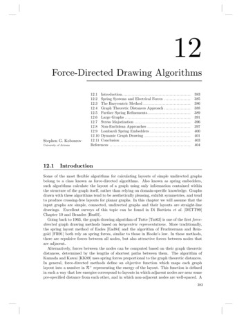
384CHAPTER 12. FORCE-DIRECTED DRAWING ALGORITHMSFigure 12.1 Examples of drawings obtained with force-directed algorithms. First row:small graphs: dodecahedron (20 vertices), C60 bucky ball (60 vertices), 3D cube mesh (216vertices). Second row: Cubes in 4D, 5D and 6D [GK02].layout for a graph is then calculated by finding a (often local) minimum of this objectivefunction; see Figure 12.1.The utility of the basic force-directed approach is limited to small graphs and results arepoor for graphs with more than a few hundred vertices. There are multiple reasons whytraditional force-directed algorithms do not perform well for large graphs. One of the mainobstacles to the scalability of these approaches is the fact that the physical model typicallyhas many local minima. Even with the help of sophisticated mechanisms for avoiding localminima the basic force-directed algorithms are not able to consistently produce good layoutsfor large graphs. Barycentric methods also do not perform well for large graphs mainly dueto resolution problems: for large graphs the minimum vertex separation tends to be verysmall, leading to unreadable drawings.The late 1990s saw the emergence of several techniques extending the functionality offorce-directed methods to graphs with tens of thousands and even hundreds of thousands ofvertices. One common thread in these approaches is the multi-level layout technique, wherethe graph is represented by a series of progressively simpler structures and laid out in reverseorder: from the simplest to the most complex. These structures can be coarser graphs (as inthe approach of Hadany and Harel [HH01], Harel and Koren [HK02], and Walshaw [Wal03],or vertex filtrations as in the approach of Gajer, Goodrich, and Kobourov [GGK04].The classical force-directed algorithms are restricted to calculating a graph layout inEuclidean geometry, typically R2 , R3 , and, more recently, Rn for larger values of n. Thereare, however, cases where Euclidean geometry may not be the best option: Certain graphsmay be known to have a structure which would be best realized in a different geometry,
12.2. SPRING SYSTEMS AND ELECTRICAL FORCES385such as on the surface of a sphere or on a torus. In particular, 3D mesh data can beparameterized on the sphere for texture mapping or graphs of genus one can be embedded ona torus without crossings. Furthermore, it has also been noted that certain non- Euclideangeometries, specifically hyperbolic geometry, have properties that are particularly well suitedto the layout and visualization of large classes of graphs [LRP95, Mun97]. With this in mind,Kobourov and Wampler describe extensions of the force-directed algorithms to Riemannianspaces [KW05].12.2Spring Systems and Electrical ForcesThe 1984 algorithm of Eades [Ead84] targets graphs with up to 30 vertices and uses amechanical model to produce “aesthetically pleasing” 2D layouts for plotters and CRTscreens. The algorithm is succinctly summarized as follows:To embed a graph we replace the vertices by steel rings and replace each edge witha spring to form a mechanical system. The vertices are placed in some initiallayout and let go so that the spring forces on the rings move the system to aminimal energy state. Two practical adjustments are made to this idea: firstly,logarithmic strength springs are used; that is, the force exerted by a spring is:c1 log(d/c2 ),where d is the length of the spring, and c1 and c2 are constants. Experienceshows that Hookes Law (linear) springs are too strong when the vertices are farapart; the logarithmic force solves this problem. Note that the springs exert noforce when d c2 . Secondly, we make nonadjacent vertices repel each other. Aninverse square law force,c3 /d2 ,where c3 is constant and d is the distance between the vertices, is suitable. Themechanical system is simulated by the following algorithm.algorithm SPRING(G:graph);place vertices of G in random locations;repeat M timescalculate the force on each vertex;move the vertex c4 (force on vertex)draw graph on CRT or plotter.The values c1 2, c2 1, c3 1, c4 0.1, are appropriate for most graphs.Almost all graphs achieve a minimal energy state after the simulation step isrun 100 times, that is, M 100.This excellent description encapsulates the essence of spring algorithms and their naturalsimplicity, elegance, and conceptual intuitiveness. The goals behind “aesthetically pleasing”layouts were initially captured by the two criteria: “all the edge lengths ought to be thesame, and the layout should display as much symmetry as possible.”The 1991 algorithm of Fruchterman and Reingold added “even vertex distribution” to theearlier two criteria and treats vertices in the graph as “atomic particles or celestial bodies,
386CHAPTER 12. FORCE-DIRECTED DRAWING ALGORITHMSexerting attractive and repulsive forces from one another.” The attractive and repulsiveforces are redefined tofa (d) d2 /k,fr (d) k 2 /d,in terms of the distance d between two vertices and the optimal distance between verticesk defined asrarea.k Cnumber of verticesThis algorithm is similar to that of Eades in that both algorithms compute attractiveforces between adjacent vertices and repulsive forces between all pairs of vertices. Thealgorithm of Fruchterman and Reingold adds the notion of “temperature” which couldbe used as follows: “the temperature could start at an initial value (say one tenth thewidth of the frame) and decay to 0 in an inverse linear fashion.” The temperature controlsthe displacement of vertices so that as the layout becomes better, the adjustments becomesmaller. The use of temperature here is a special case of a general technique called simulatedannealing, whose use in force-directed algorithms is discussed later in this chapter. Thepseudo-code for the algorithm by Fruchterman and Reingold, shown in Figure 12.2 providesfurther insight into the workings of a spring-embedder.Each iteration the basic algorithm computes O( E ) attractive forces and O( V 2 ) repulsive forces. To reduce the quadratic complexity of the repulsive forces, Fruchterman andReingold suggest using a grid variant of their basic algorithm, where the repulsive forces between distant vertices are ignored. For sparse graphs, and with uniform distribution of thevertices, this method allows a O( V ) time approximation to the repulsive forces calculation.This approach can be thought of as a special case of the multi-pole technique introduced inn-body simulations [Gre88] whose use in force-directed algorithms will be further discussedlater in this chapter.As in the paper by Eades [Ead84] the graphs considered by Fruchterman and Reingoldare small graphs with less than 40 vertices. The number of iterations of the main loop isalso similar at 50.12.3The Barycentric MethodHistorically, Tutte’s 1963 barycentric method [Tut63] is the first “force-directed” algorithmfor obtaining a straight-line, crossings free drawing for a given 3-connected planar graph.Unlike almost all other force-directed methods, Tutte’s guarantees that the resulting drawing is crossings-free; moreover, all faces of the drawing are convex.The idea behind Tutte’s algorithm, shown in Figure 12.3, is that if a face of the planargraph is fixed in the plane, then suitable positions for the remaining vertices can be found bysolving a system of linear equations, where each vertex position is represented as a convexcombination of the positions of its neighbors. This algorithm be considered a force-directedmethod as summarized in Di Battista et al. [DETT99].In this model the force due to an edge (u, v) is proportional to the distance betweenvertices u and v and the springs have ideal length of zero; there are no explicit repulsiveforces. Thus the force at a vertex v is described byXF (v) (pu pv ),(u,v) Ewhere pu and pv are the positions of vertices u and v. As this function has a trivial minimumwith all vertices placed in the same location, the vertex set is partitioned into fixed and free
12.3. THE BARYCENTRIC METHOD387area: W L; {W and L are the width and length of the frame}G : p(V, E); {the vertices are assigned random initial positions}k : area/ V ;function fa (x) : begin return x2 /k end;function fr (x) : begin return k 2 /x end;for i : 1 to iterations do begin{calculate repulsive forces}for v in V do begin{each vertex has two vectors: .pos and .dispv.disp : 0;for u in V doif (u 6 v) then begin{δ is the difference vector between the positions of the two vertices}δ : v.pos u.pos;v.disp : v.disp (δ/ δ ) fr ( δ )endend{calculate attractive forces}for e in E do begin{each edges is an ordered pair of vertices .vand.u}δ : e.v.pos e.u.pos;e.v.disp : e.v.disp (δ/ δ ) fa ( δ );e.u.disp : e.u.disp (δ/ δ ) fa ( δ )end{limit max displacement to temperature t and prevent from displacementoutside frame}for v in V do beginv.pos : v.pos (v.disp/ v.disp ) min(v.disp, t);v.pos.x : min(W/2, max( W/2, v.pos.x));v.pos.y : min(L/2, max( L/2, v.pos.y))end{reduce the temperature as the layout approaches a better configuration}t : cool(t)endFigure 12.2Pseudo-code for the algorithm by Fruchterman and Reingold [FR91].vertices. Setting the partial derivatives of the force function to zero results in independentsystems of linear equations for the x-coordinate and for the y-coordinate.The equations in the for-loop are linear and the number of equations is equal to thenumber of the unknowns, which in turn is equal to the number of free vertices. Solving theseequations results in placing each free vertex at the barycenter of its neighbors. The systemof equations can be solved using the Newton-Raphson method. Moreover, the resultingsolution is unique.One significant drawback of this approach is the resulting drawing often has poor vertexresolution. In fact, for every n 1, there exists a graph, such that the barycenter methodcomputes a drawing with exponential area [EG95].
388CHAPTER 12. FORCE-DIRECTED DRAWING ALGORITHMSBarycenter-DrawInput: G (V, E); a partition V V0 V1 of V into a set V0 of at least threefixed vertices and a set V1 of free vertices; a strictly convex polygon P with V0 verticesOutput: a position pv for each vertex of V , such that the fixed vertices form aconvex polygon P .1. Place each fixed vertex u V0 at a vertex of P , and each free vertex at theorigin.2. repeatforeach free vertex v V1 doxv yv 1deg(v)1deg(v)XxuXyu(u,v) E(u,v) Euntil xv and yv converge for all free vertices v.Figure 12.312.4Tutte’s barycentric method [Tut63]. Pseudo-code from [DETT99].Graph Theoretic Distances ApproachThe 1989 algorithm of Kamada and Kawai [KK89] introduced a different way of thinkingabout “good” graph layouts. Whereas the algorithms of Eades and Fruchterman-Reingoldaim to keep adjacent vertices close to each other while ensuring that vertices are not tooclose to each other, Kamada and Kawai take graph theoretic approach:We regard the desirable geometric (Euclidean) distance between two vertices inthe drawing as the graph theoretic distance between them in the correspondinggraph.In this model, the “perfect” drawing of a graph would be one in which the pair-wise geometric distances between the drawn vertices match the graph theoretic pairwise distances,as computed by an All-Pairs-Shortest-Path computation. As this goal cannot always beachieved for arbitrary graphs in 2D or 3D Euclidean spaces, the approach relies on settingup a spring system in such a way that minimizing the energy of the system corresponds tominimizing the difference between the geometric and graph distances. In this model thereare no separate attractive and repulsive forces between pairs of vertices, but instead if apair of vertices is (geometrically) closer/farther than their corresponding graph distance thevertices repel/attract each other. Let di,j denote the shortest path distance between vertexi and vertex j in the graph. Then li,j L di,j is the ideal length of a spring betweenvertices i and j, where L is the desirable length of a single edge in the display. Kamada
12.5. FURTHER SPRING REFINEMENTS389and Kawai suggest that L L0 / maxi j di,j , where L0 is the length of a side of the displayarea and maxi j di,j is the diameter of the graph, i.e., the distance between the farthestpair of vertices. The strength of the spring between vertices i and j is defined aski,j K/d2i,j ,where K is a constant. Treating the drawing problem as localizing V n particlesp1 , p2 , . . . , pn in 2D Euclidean space, leads to the following overall energy function:E nX1ki,j ( pi pj li,j )2 .2i 1 j i 1n 1XThe coordinates of a particle pi in the 2D Euclidean plane are given by xi and yi whichallows us to rewrite the energy function as follows:E nqX12 2li,j (xi xj )2 (yi yj )2 .ki,j (xi xj )2 (yi yj )2 li,j2i 1 j i 1n 1XThe goal of the algorithm is to find values for the variables that minimize the energyfunction E(x1 , x2 , . . . , xn , y1 , y2 , . . . , yn ). In particular, at a local minimum all the partialderivatives are equal to zero, and which corresponds to solving 2n simultaneous non-linearequations. Therefore, Kamada and Kawai compute a stable position one particle pm ata time. Viewing E as a function of only xm and ym a minimum of E can be computedusing the Newton-Raphson method. At each step of the algorithm the particle pm with thelargest value of m is chosen, wheres 2 2 E E m . xm ymPseudo-code for the algorithm by Kamada and Kawai is shown in Figure 12.4.The algorithm of Kamada and Kawai is computationally expensive, requiring an All-PairShortest-Path computation which can be done in O( V 3 )time using the Floyd-Warshall algorithm or in O( V 2 log V E V ) using Johnson’s algorithm; see the All-Pairs-ShortestPath chapter in an algorithms textbook such as [CLRS90]. Furthermore, the algorithmrequires O( V 2 ) storage for the pairwise vertex distances. Despite the higher time andspace complexity, the algorithm contributes a simple and intuitive definition of a “good”graph layout: A graph layout is good if the geometric distances between vertices closelycorrespond to the underlying graph distances.12.5Further Spring RefinementsEven before the 1984 algorithm of Eades, force-directed techniques were used in the contextof VLSI layouts in the 1960s and 1970s [FCW67, QB79]. Yet, renewed interest in forcedirected graph layout algorithms brought forth many new ideas in the 1990s. Frick, Ludwig,and Mehldau [FLM95] add new heuristics to the Fruchterman-Reingold approach. In particular, oscillation and rotations are detected and dealt with using local instead of globaltemperature. The following year Bruß and Frick [BF96] extended the approach to layoutsdirectly in 3D Euclidean space. The algorithm of Cohen [Coh97] introduced the notion ofan incremental layout, a precursor of the multi-scale methods described in Section 12.6.
390CHAPTER 12. FORCE-DIRECTED DRAWING ALGORITHMScompute di,j for 1 i 6 j n;compute li,j for 1 i 6 j n;compute ki,j for 1 i 6 j n;initialize p1 , p2 , . . . , pn ;while (maxi i ǫ)let pm be the particle satisfying m maxi i ;while ( m ǫ)compute δx and δy by solving the following system of equations: 2 E (t) (t) 2E E (t) (t)(t)(x,y)δx (x(t)(x , y );mmm , ym )δy 2 xm xm ym xm m m 2E E (t) (t) 2 E (t) (t)(t)(xm , ym )δy (x(t)(x , y )m , ym )δx 2 ym xm ym ym m mxm : xm δx;ym : ym δy;Figure 12.4Pseudo-code for the algorithm by Kamada and Kawai [KK89].The 1997 algorithm of Davidson and Harel [DH96] adds additional constraints to thetraditional force-directed approach in explicitly aiming to minimize the number of edgecrossings and keeping vertices from getting too close to non-adjacent edges. The algorithm uses the simulated annealing technique developed for large combinatorial optimization [KGV83]. Simulated annealing is motivated by the physical process of cooling moltenmaterials. When molten steel is cooled too quickly it cracks and forms bubbles making itbrittle. For better results, the steel must be cooled slowly and evenly and this process isknown as annealing in metallurgy. With regard to force-directed algorithms, this process issimulated to find local minima of the energy function. Cruz and Twarog [CT96] extendedthe method by Davidson and Harel to three-dimensional drawings.Genetic algorithms for force-directed placement have also been considered. Genetic algorithms are a commonly used search technique for finding approximate solutions to optimization and search problems. The technique is inspired by evolutionary biology in generaland by inheritance, mutation, natural selection, and recombination (or crossover), in particular; see the survey by Vose [Vos99]. In the context of force-directed techniques forgraph drawing, the genetic algorithms approach was introduced in 1991 by Kosak, Marksand Shieber [KMS91]. Other notable approaches in the direction include that of Branke,Bucher, and Schmeck [BBS97].In the context of graph clustering, the LinLog model introduces an alternative energymodel [Noa07]. Traditional energy models enforce small and uniform edge lengths, whichoften prevent the separation of nodes in different clusters. As a side effect, they tendto group nodes with large degree in the center of the layout, where their distance to theremaining nodes is relatively small. The node-repulsion LinLog and edge- repulsion LinLogmodels group nodes according to two well-known clustering criteria: the density of thecut [LR88] and the normalized cut [SM00].
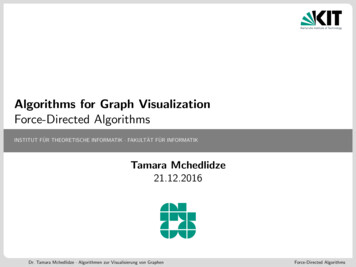
12.6. LARGE GRAPHS12.6391Large GraphsThe first force-directed algorithms to produce good layouts for graphs with more than 1000vertices is the 1999 algorithm of Hadany and Harel [HH01]. They introduced the multiscale technique as a way to deal with large graphs and in the following year four relatedbut independent force-directed algorithms for large graphs were presented at the AnnualSymposium on Graph Drawing. We begin with Hadany and Harel’s description on themulti-scale method :A natural strategy for drawing a graph nicely is to first consider an abstraction,disregarding some of the graph’s fine details. This abstraction is then drawn,yielding a “rough” layout in which only the general structure is revealed. Thenthe details are added and the layout is corrected. To employ such a strategyit is crucial that the abstraction retains essential features of the graph. Thus,one has to define the notion of coarse-scale representations of a graph, in whichthe combinatorial structure is significantly simplified but features important forvisualization are well preserved. The drawing process will then “travel” betweenthese representations, and introduce multi-scale corrections. Assuming we havealready defined the multiple levels of coarsening, the general structure of ourstrategy is as follows:1. Perform fine-scale relocations of vertices that yield a locally organized configuration.2. Perform coarse-scale relocations (through local relocations in the coarse representations), correcting global disorders not found in stage 1.3. Perform fine-scale relocations that correct local disorders introduced by stage 2.Hadany and Harel suggest computing the sequence of graphs by using edge contractionsso as to preserve certain properties of the graph. In particular, the goal is to preserve threetopological properties: cluster size, vertex degrees, and homotopy. For the coarse-scalerelocations, the energy function for each graph in the sequence is that of Kamada and Kawai(the pairwise graph distances are compared to the geometric distances in the current layout).For the fine-scale relocations, the authors suggest using force-directed calculations as thoseof Eades [Ead84], Fruchterman-Reingold [FR91], or Kamada-Kawai [KK89]. While theasymptotic complexity of this algorithm is similar to that of the Kamada-Kawai algorithm,the multi-scale approach leads to good layouts for much larger graphs in reasonable time.The algorithm of Harel and Koren [HK02] took force-directed algorithms to graphs with15,000 vertices. This algorithm is similar to the algorithm of Hadany and Harel, yet usesa simpler coarsening process based on a k-centers approximation, and a faster fine-scalebeautification. Given a graph G (V, E), the k-centers problem asks to find a subset ofthe vertex set V ′ V of size k, so as to minimize the maximum distance from a vertex toV ′ : min u V maxu V,v V ′ dist(u, v). While k-centers is an NP-hard problem, Harel andKoren use a straightforward and efficient 2-approximation algorithm that relies on BreadthFirst Search [Hoc96]. The fine-scale vertex relocations are done using the Kamada-Kawaiapproach. The Harel and Koren algorithm is summarized in Figure 12.5.
392CHAPTER 12. FORCE-DIRECTED DRAWING ALGORITHMSLayout(G(V, E))% Goal: Find L, a nice layout of G% Constants:% Rad[ 7] – determines radius of local neighborhoods% Iterations[ 4] – determines number of iterations in local beautification% Ratio[ 3] – ratio between number of vertices in two consecutive levels% MinSize[ 10] – size of the coarsest graphCompute the all-pairs shortest path length: dV VSet up a random layout Lk M inSizewhile k V docenters K-Centers(G(V, E), k)radius maxv centers minu centers {dvu } RadLocalLayout(dcenters centers , L(centers), radius, Iterations)for every v V doL(v) L(center(v)) randk kRatioreturn LK-Centers(G(V, E), k)% Goal: Find a set S V of size k, such that maxv V mins S {dsv } isminimized.S {v} for some arbitrary v Vfor i 2 to k do1. Find the vertex u farthest away from S(i.e., such that mins S {dus } mins S {dws }, w V )2. S S {u}return SLocalLayout(dV V , L, k, Iterations)% Goal: Find a locally nice layout L by beautifying k-neighborhoods% dV V : all-pairs shortest path length% L: initialized layout% k: radius of neighborhoodsfor i 1 to Iterations V do1. Choose the vertex v with the maximal kv2. Compute δvk as in Kamada-Kawai3. L(v) L(v) (δvk (x), δvk (y))endFigure 12.5Pseudo-code for the algorithm by Harel and Koren [HK02].
12.6. LARGE GRAPHS393Main Algorithmcreate a filtration V : V0 V1 . . . Vk for i k to 0 dofor each v Vi Vi 1 dofind vertex neighborhood Ni (v), Ni 1 (v), . . . , N0 (v)find initial position pos[v] of vrepeat rounds timesfor each v Vi docompute local temperature heat[v] disp[v] heat[v] · FNi (v)for each v Vi dopos[v] pos[v] disp[v]add all edges e EFigure 12.6Pseudo-code for the algorithm by Gajer et al. [GGK04].The 2000 algorithm of Gajer et al. [GGK04], shown in Figure 12.6, is also a multiscale force-directed algorithm but introduces several ideas to the realm of multi-scale forcedirected algorithms for large graphs. Most importantly, this approach avoids the quadraticspace and time complexity of previous force-directed approaches with the help of a simplercoarsening strategy. Instead of computing a series of coarser graphs from the given largegraph G (V, E), Gajer et al. produce a vertex filtration V : V0 V1 . . . Vk ,where V0 V (G) is the original vertex set of the given graph G. By restricting the numberof vertices considered in relocating any particular vertex in the filtration and ensuring thatthe filtration has O(log V ) levels an overall running time of O( V log2 V ) is achieved.Filtrations based on graph centers (as in Harel and Koren [HK02]) and maximal independentsets are considered. V V0 V1 . . . Vk , is a maximal independent set filtrationof G if Vi is a maximal subset of Vi 1 for which the graph distance between any pair of itselements is greater than or equal to 2i .In the GRIP system [GK02], Gajer et al. add to the filtration and neighborhood calculations of [GGK04]: they introduce the idea of realizing the graph in high-dimensionalEuclidean space and obtaining 2D or 3D projections at the end. The algorithm also relieson intelligent initial placement of vertices based on graph theoretic distances, rather thanon random initial placement. Finally, the notion of cooling is re-introduced in the contextof multi-scale force-directed algorithms. The GRIP system produces high-quality layouts, asillustrated in Figure 12.7.Another multilevel algorithm is that of Walshaw [Wal03]. Instead of relying on theKamada-Kawai type force interactions, this algorithm extends the grid variant of FruchtermanReingold to a multilevel algorithm. The coarsening step is based on repeatedly collapsing maximally independent sets of edges, and the fine-scale refinements are based onFruchterman-Reingold force calculations. This O( V 2 ) algorithm is summarized in Figure 12.8.
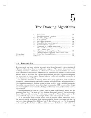
394CHAPTER 12. FORCE-DIRECTED DRAWING ALGORITHMSThe fourth 2000 multilevel force-directed algorithm is due to Quigley and Eades [QE00].This algorithm relies on the Barnes-Hut n-body simulation method [BH86] and reducesrepulsive force calculations to O( V log V ) time instead of the usual O( V 2 ). Similarly,the algorithm of Hu [Hu05] combines the multilevel approach with the n-bosy simulationmethod, and is implemented in the sfdp drawing engine of GraphViz [EGK 01].One possible drawback to this approach is that the running time depends on the distribution of the vertices. Hachul and Jünger [HJ04] address this problem in their 2004 multilevelalgorithm.Figure 12.7 Drawings from GRIP. First row: knotted meshes of 1600, 2500, and 10000vertices. Second row: Sierpinski graphs of order 7 (1,095 vertices), order 6 (2,050 vertices),3D Sierpinski of order 7 (8,194 vertices) [GK02].
12.6. LARGE GRAPHSfunction fg (x, w): begin return Cwk 2 /x endfunction fl (x, d, w): begin return {(x k)/d} fg (x, w) endt : t0 ;P osn : N ewP osn;while (converged 6 1) beginconverged : 1;for v V beginOldP osn[v] N ewP osn[v]endfor v V begin{initialize D, the vector of displacements of v}D : 0;{calculate global (repulsive) forces}for u V, u 6 v begin : P osn[u] P osn[v];D : D ( / Delta ) fg ( , u );end{calculate local (spring) forces }for u Γ(v) begin : P osn[u] P osn[v];D : D ( / Delta ) fl ( , Γ(v) , u );end{reposition v}N ewP osn[v] N ewP osn[v] (D/ D ) min(t, D ); : N ewP osn[v] OldP osn[v];if ( k tol)converged : 0;end{reduce the temperature to reduce the maximum movement}t : cool(t);endFigure 12.8Pseudo-code for the algorithm by Walshaw [Wal03].395
39612.7CHAPTER 12. FORCE-DIRECTED DRAWING ALGORITHMSStress MajorizationMethods that exploit fast algebraic operations offer another practical way to deal withlarge graphs. Stress minimization has been proposed and implemented in the more generalsetting of multidimensional scaling (MDS) [Kru64]. The function describing the stress issimilar to the layout energy function of Kamada-Kawai from Section 12.4:E nX1ki,j ( pi pj li,j )
for obtaining a straight-line, crossings free drawing for a given 3-connected planar graph. Unlike almost all other force-directed methods, Tutte's guarantees that the resulting draw-ing is crossings-free; moreover, all faces of the drawing are convex. The idea behind Tutte's algorithm, shown in Figure 12.3, is that if a face of the planar