Transcription
Lecture notes on Transportation and Assignment Problem (BBE (H) QTM paper of DelhiUniversity)Transportation and Assignment ProblemsThe transportation model is a special class of linear programs. It received this name because many of itsapplications involve determining how to optimally transport goods. However, some of its importantapplications (eg production scheduling) actually have nothing to do with transportation.The second type of problem is assignment problem. It involves such applications as assigning people totasks. Although its applications appear to be quite different from those for the transportation, we shallsee the assignment problem can be viewed as a special type of transportation problem.Application of the transportation and assignment problem tend to require a very large number ofconstraints and variables, so straightforward computer applications of simplex method may require anexorbitant computational effort. Fortunately, a key characteristic of these problems is that most of the aijcoefficient in the constraints are zeros, and the relatively few non zero coefficient appear in a distinctivepattern. As a result, it has been possible to develop special streamlined algorithms that achieve dramaticcomputational savings by exploiting this special structure of the problem. Therefore, it is important tobecome sufficiently familiar with these special types of problems that you can recognise them when theyarises and apply the proper computational procedure.Transportation problemAs pointed out above that many applications of TP deals with transportation of a commodity fromsource to destination. Therefore I will use prototype example to explain the TP.Example- Suppose XYZ Pvt Ld produce good X. The production take place at 3 place- S1, S2 and S3.From these production places, company supplies the X to its warehouses, which are located near itsdemand centre. The shipping cost or transportation cost from different production place to warehouses isgiven table 1http://rajkumar2850.weebly.com/, Rajkumar, Assistant Professor, College of Vocational Studies,Delhi. Email- rajkumar dse@outlook.comNote-This notes are not substitutes of Text books. Please refer to your text book.1
Lecture notes on Transportation and Assignment Problem (BBE (H) QTM paper of DelhiUniversity)Table 1Shpping cost per 5S399568238868510080657085AllocationSi represents the production place(sources) and Wi represents the warehouses (destinations).We can represent the above problem with network diagram as followingIn above fig, the arrows shows the possible routes for transportation, where the number next to eacharrow is the shipping cost per unit for that route. A square bracket net to each location gives the numberof units to be shipped out of that location (so that the allocation into each warehouse is given as anegative number)http://rajkumar2850.weebly.com/, Rajkumar, Assistant Professor, College of Vocational Studies,Delhi. Email- rajkumar dse@outlook.comNote-This notes are not substitutes of Text books. Please refer to your text book.2
Lecture notes on Transportation and Assignment Problem (BBE (H) QTM paper of DelhiUniversity)We can also represent the above problem in term of linear programming.With above cost structure, the linear programming problem of the firm will beThe table 2 shows the constraint coefficients. As I will explain in class, it is the special structure in thepattern of these coefficients that distinguishes this problem as a transportation problem, not its context.Table ly.com/, Rajkumar, Assistant Professor, College of Vocational Studies,Delhi. Email- rajkumar dse@outlook.comNote-This notes are not substitutes of Text books. Please refer to your text book.3
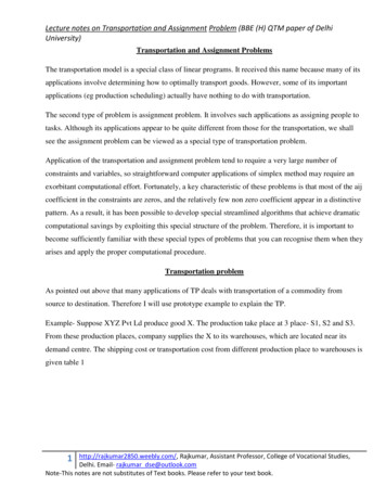
Lecture notes on Transportation and Assignment Problem (BBE (H) QTM paper of DelhiUniversity)The supply constraints also called as Source constraints and the Demand constraints are also called asWarehouse constraints.It becomes very clear from above example that coefficient table of transportation problem have veryspecial structure. We can show the same pattern for general transportation problem with sourcei 1,2, m and destination j 1,2, n.The unit cost of this general transportation problem will becost per unit distributeddestinationsupply1source2 .n1 c11c12c1nS12 c21c22c2nS2cm1cm2cmnSmd2dn.mdemand d1In above table c11 represents the unit cost of transportation from source 1 to destination 1. In the sameway, c12 repesents the unit cost of transportation from source 1 to destination 2.The mathematical formation for this problem will beMin Z i j cijxijSubject to i xij si j xij djxij 0 for all i and j.http://rajkumar2850.weebly.com/, Rajkumar, Assistant Professor, College of Vocational Studies,Delhi. Email- rajkumar dse@outlook.comNote-This notes are not substitutes of Text books. Please refer to your text book.4
Lecture notes on Transportation and Assignment Problem (BBE (H) QTM paper of DelhiUniversity)In transportation model we make following two assumption. The requirement assumption- Each sources has a fixed supply of units, where this entire supplymust be distributed to the destinations. Similarly, each destination has a fixed demand for units,where this entire demand must be received from the sources. The cost assumptions- the cost of distributing units from any particular source to any particulardestination is directly proportional to the number of units distributed. Therefore, the cost is justthe unit cost of distribution times the number of units distributed.Note that the resulting table of constraint coefficients has the special structure shown in following table.Table 3So any problem (whether involving transportation or not) fits the model for a transportation problem if itcan be described completely in terms of a parameter table like above table and it satisfies both therequirement assumptions and the cost assumption. The objective is to minimise the total cost ofdistributing the units. All the parameters of the model are included in this table.Any linear programming problem that fits this special formulation is of thetransportation problem type, regardless of its physical context.http://rajkumar2850.weebly.com/, Rajkumar, Assistant Professor, College of Vocational Studies,Delhi. Email- rajkumar dse@outlook.comNote-This notes are not substitutes of Text books. Please refer to your text book.5
Lecture notes on Transportation and Assignment Problem (BBE (H) QTM paper of DelhiUniversity)Solution PropertiesThe feasible solution property- a transportation problem will have feasible solutions if and only if si dj model is balanced.i.e. total supply must be equal to total demand.Integer solution property- for transportation problems where every si and dj have an integer value, allthe basic variables (allocations) in every basic feasible solution (including an optimal one) also haveinteger values.Basic Terminology1. Rim Requirement- the supply and demand requirements at various source and destinations iscalled Rim requirement.2. Feasible Solution- A feasible solution to a transportation problem is a set of non-negativeallocations, xij, that satisfies the rim (row and column) restrictions.3. Basic Feasible solution- A feasible solution is called a basic feasible solution if it contains nomore than m n-1 non negative allocations where m is the number of rows and n is the number ofcolumns of the transportation problem.4. Degenerated basic feasible- A basic solution that contains less than m n-1 non-negativeallocations in independent positions. The allocation are said to be independent positions, if it isnot possible to form a closed path (loop) means by allowing horizontal and vertical lines and ifall the corner cells are occupied. (explanation in class)5. Non-degenerated basic feasible- A basic solution that contains exactly m n-1 non-negativeallocations is called degenerated basic feasible solution.6. Optimal Solution- A feasible solution (non necessarily basic) is said to be optimal if it minimises(maximises) the transportation cost (profit).7. Balance and Unbalance Transportation Problem-If the total demand is equal to total supply thenTP is called balance TP, otherwise it is unbalance TP8. Occupied and Unoccupied cells- the allocated cells in the transportation cells occupied cells andempty cells are called non-occupied cells.http://rajkumar2850.weebly.com/, Rajkumar, Assistant Professor, College of Vocational Studies,Delhi. Email- rajkumar dse@outlook.comNote-This notes are not substitutes of Text books. Please refer to your text book.6
Lecture notes on Transportation and Assignment Problem (BBE (H) QTM paper of DelhiUniversity)The Transportation AlgorithmAlgorithm- A process or set of rules to be followed incalculations or other problem solving operationsThe transportation algorithm follows the exact steps of the simplex method. However, instead of usingthe regular simplex tableau, we take advantage of the special structure of the transportation model toorganise the computations in a more convenient form.Steps- the steps of the transportation algorithm are exact parallels of the simplex algorithm,Step 1- Determine a starting basic feasible solution, andStep 2- use the optimality condition of the simplex method to determine the entering variable fromamong all the non basic variables. If the optimality condition is satisfied, stop. Otherwise go to step 3Step 3- use the feasibility condition of the simplex method to determine the leaving variable from amongall the current basic variables, and find the new basic solution. Return to step 2.Step 1: Determination of the starting solutionA general transportation model with m sources and n destinations has m n constraint equations, one foreach source and each destination. However, because the transportation model is always balanced (sumof the supply sum of the demad), one of these equations is redundant. Thus, the model has m n-1independent constraint equations, which means that the starting solution basic solution consists of m n1 independent equations, which means that the starting basic solution consists of m n-1 basic variables.The special structure of the transportation problem allows securing a nonartificial starting basic solutionusing one of three methods(1) Least cost method(2) Vogel approximation method.Above methods differ in the quality of the starting basic solution they produce, in the sense that a betterstarting solution yields a smaller objective value.http://rajkumar2850.weebly.com/, Rajkumar, Assistant Professor, College of Vocational Studies,Delhi. Email- rajkumar dse@outlook.comNote-This notes are not substitutes of Text books. Please refer to your text book.7
Lecture notes on Transportation and Assignment Problem (BBE (H) QTM paper of DelhiUniversity)Least cost methodStep I write the transportation problem in a tabular formStep II Assigns as much as possible to the cell with the smallest unit cost.Step III the satisfied row or column is crossed out and the amount of supply and demand are adjustedaccordingly. If both a row and a column are satisfied simultaneously, only one is crossed out.Step IV Look for the uncrossed out cell with the smallest unit cost and repeat the process until exactlyone row or column is left uncrossed out.Vogel’s approximation method (VAM)VAM is an improved version of the least cost method that generally, but not always, produces moreefficient starting solutions.Step I Write the TP in the tabular formStep II For each row (column), determine a penalty measure by subtracting the smallest unit costelement in the row (column) from the next smallest unit cost element in the same row (column)Step III Identify the row or column with the largest penalty. Break ties arbitrarily. Allocate as much aspossible to the variable with the least unit cost in the selected row or column. Adjust the supply anddemand, and cross out the satisfied row or column. If a row and a column are satisfied simultaneously,only one of the two is crossed out, and the remaining row (column) is assigned zero supply (demand).Step IV (a) if exactly one row or column with zero supply or demand remains uncrossed out, stop.(b) if one row (column) with positive supply (demand) remains uncrossed out, determine thebasic variable in the row (column) by the least cost method. Stop(c) if all the uncrossed out rows and columns have (remaining) zero supply and demand,Determine the zero basic variables by the least cost method. Stop(d) Otherwise, go to step IIVAM is popular because it is relatively easy to implement by hand.http://rajkumar2850.weebly.com/, Rajkumar, Assistant Professor, College of Vocational Studies,Delhi. Email- rajkumar dse@outlook.comNote-This notes are not substitutes of Text books. Please refer to your text book.8
Lecture notes on Transportation and Assignment Problem (BBE (H) QTM paper of DelhiUniversity)The penalty in VAM represents the minimum extra unit cost incurred by failing to make an allocation tothe cell having the smallest unit in that row or column, this criterion does take costs into account in aneffective way.Numerical Example----------------Unbalanced Transportation ModelA necessary and sufficient condition for the existence of feasible solution to the general transportationproblem is that the total demand must equal the total supply. However, sometimes there may be moredemand than the supply and vice versa in which case the problem is said to be unbalanced. If may occurin the following situation1. SS DD2. DD SSIn case I, we introduce a dummy destination in the transportation table. The cost of transportating to thisdestination are all set equal to zero. The requirement at this dummy destination is then assumed to beequal toSS – DDIn case 2, we introduce a dummy source in the transportation table. The cost of transporting from thissource to any destinations is all set equal to zero. The availability at this dummy source is assumed to beequal to DD – SS.Step 2 and 3: Test of optimality and optimal solutionOnce an initial solution is obtained, the next step is to check its optimality. An optimal solution is onewhere there is no other set of transportation route (allocations) that will further reduce the totaltransportation cost. Thus we have to evaluate each unoccupied cell (represents unused route) in thetransportation table in terms of an opportunity of reducing total transportation cost.There are two methods to check optimality1. Stepping Stone Method2. Modified distribution (MODI)http://rajkumar2850.weebly.com/, Rajkumar, Assistant Professor, College of Vocational Studies,Delhi. Email- rajkumar dse@outlook.comNote-This notes are not substitutes of Text books. Please refer to your text book.9
Lecture notes on Transportation and Assignment Problem (BBE (H) QTM paper of DelhiUniversity)Stepping Stone MethodThis is a procedure for determining the potential of improving upon each of the non-basic variables interms of the objective function. To determine this potential, each of the non-basic variables is consideredone by one. For each such cell, we find what effect on the total cost would be if one unit is assigned tothis cell. With this information, then, we come to know whether the solution is optimal or not. If not, weimprove that solution.We can summarise the Stepping Stone method in following steps1. Construct a transportation table with a given unit cost of transportation along with the rimconditions2. Determine a initial basic feasible solution (allocation) using a suitable method as discussedearlier3. Evaluate all unoccupied cells for the effect of transferring one unit from an occupied cell to theunoccupied cell. This transfer is made by forming a closed path that retains the SS and DDcondition of the problem4. Check the sign of each of the net change in the unit transportation costs. If the net changes areplus or zero, then the an optimal solution has been arrived at, otherwise go to step 55. Select the unoccupied cell with most negative net change among all unoccupied cells.6. Assign an many units as possible to unoccupied cell satisfying rim conditions. The maximumnumber of units to be assigned are equal to the smaller circled number among the occupied cellswith the minus value in a closed path.7. Go to step 3, and repeat the problem until all unoccupied cells are evaluated and the net changeresult in positive or zero.Numerical Example – in ClassModified Distribution (MODI) methodMODI method is based on the concept of duality. To explain this, we will use prototype example.http://rajkumar2850.weebly.com/, Rajkumar, Assistant Professor, College of Vocational Studies,Delhi. Email- rajkumar dse@outlook.comNote-This notes are not substitutes of Text books. Please refer to your text book.10
Lecture notes on Transportation and Assignment Problem (BBE (H) QTM paper of DelhiUniversity)Suppose the unit cost of transportation of XYZ company is given in following 2S2d1d2DemandThe simplex formulation of this problem will beMinZ c11x11 c12x12 c21x21 c22x22s.tx11 x12 s1x21 x11 x22x21x12 s2 d1 x22 d2For duality, introduce ui for supply constraint and vj for demand constraint.DualMaxZ u1s1 u2s2 v1d1 v2d2u1 v1 c11s.t.u1 v2 c12u2 v1 c21u2 v2 c22so in case of general transportation model:http://rajkumar2850.weebly.com/, Rajkumar, Assistant Professor, College of Vocational Studies,Delhi. Email- rajkumar dse@outlook.comNote-This notes are not substitutes of Text books. Please refer to your text book.11
Lecture notes on Transportation and Assignment Problem (BBE (H) QTM paper of DelhiUniversity)MinZ i j cijxijSubject to i xij si j xij dj.xij 0 for all i and jThe dual will beMinZ i uisi j vjdjui vj cij for all i and jui , vj 0 for all i and jfrom economic interpretation, ui vj implied cost (ui denotes the location rent and vj denotes themarket price) and cij actual costThe variable xij form an optimal solution to the given transportation providedi.Solution xij is feasible for all (i,j) with respect to original transportation model,ii.(cij - ui - vj) xij 0 for all i and j. This condition is known as complementary slackness fortransportation problem.The last condition indicates thata. If xij 0 and is feasible then cij - ui - vj 0so cij ui vj for each occupied cellb. If xij 0 and is feasible then cij - ui - vj 0so cij ui vj for each occupied cell.http://rajkumar2850.weebly.com/, Rajkumar, Assistant Professor, College of Vocational Studies,Delhi. Email- rajkumar dse@outlook.comNote-This notes are not substitutes of Text books. Please refer to your text book.12
Lecture notes on Transportation and Assignment Problem (BBE (H) QTM paper of DelhiUniversity)If cij ui vj i.e. actual cost implied cost, then it is not desirable to have xij 0 in the solutionmix because it will increase transportation costIf cij ui vj i.e. actual cost implied cost, then it is desirable to have xij 0 in the solution mixbecause it will decrease transportation cost.Define dij cij -(ui vj) for all i and j.So if dij 0 then solution is not optimal. In sum, we follow following steps in MODI method1. For an initial basic feasible solution with (m n-1) occupied cells, calculate ui and vj for row andcolumnsTo start with, any one of ui’s and vj is assigned the value zero. Then complete the calculation ofui’s and vj’s for other rows and columns by using the relationcij ui vj for all occupied cells2. For unoccupied cells, calculate opportunity cost dij by using the relationship dij cij –( ui vj )for all i and j3. Examine sign of each diji.If dij 0 then current basic feasible solution is optimalii.If dij 0 then current basic feasible solution will remain unaffected but an alternativesolution existiii.If one or more dij 0 the solution is not optimal.iv.4. Reallocation of units by allocating units to the unoccupied cell, and calculate the newtransportation cost.5. Test the revised solution for optimality. The procedure terminates when all dij 0 forunoccupied cells.Numerical example---- in classhttp://rajkumar2850.weebly.com/, Rajkumar, Assistant Professor, College of Vocational Studies,Delhi. Email- rajkumar dse@outlook.comNote-This notes are not substitutes of Text books. Please refer to your text book.13
Lecture notes on Transportation and Assignment Problem (BBE (H) QTM paper of DelhiUniversity)Assignment ProblemThe AP is a special type of LPP where assignees are being assigned to perform task. For example, theassignees might be employees who need to be given work assignments. However, the assignees mightnot be people. They could be machines or vehicles or plants or even time slots to be assigned tasks.To fit the definition of an assignment problem, the problem need to formulate in a way that satisfies thefollowing assumptions1. The number of assignees and the number of tasks are the same2. Each assignees is to be assigned to exactly one task3. Each task is to performed by exactly one assignee4. There is a cost cij associated with assignee i performing task j.5. The objective is to determine how all n assignments should be made to minimise the total cost.Any problem satisfying all these assumptions can be solved extremely efficiently by algorithm designedspecifically for assignment problem.Mathematical formThe mathematical model for the assignment problem uses the following decision variablesXij 1 if assignee(worker) i perform task j 0 if not.Thus each xij is a binary variable (it has value 0 or 1). Lets Z denots the total cost, the assignmentproblem model isMin Z i j cij xijSubject to ixij 1 for i 1.n jxij 1 for j 1.nhttp://rajkumar2850.weebly.com/, Rajkumar, Assistant Professor, College of Vocational Studies,Delhi. Email- rajkumar dse@outlook.comNote-This notes are not substitutes of Text books. Please refer to your text book.14
Lecture notes on Transportation and Assignment Problem (BBE (H) QTM paper of DelhiUniversity)Xij 0 for all i and j.The first set of functional constraints specifies that each assignee is to perform exactly one task, whereasthe second set requires each task to be performed by exactly one assignee.TP & APIn comparison to TP, in AP we have following restrictions1. Number of sources (m) number of destinations (n)2. Each supply (Si) 13. Each demand (di) 1Because assignment model is special case of transportation model so we can solve assignment problemdirectly as regular transportation model. Nevertheless, the fact that all the supply and demand amountsequal 1 has led to the development of a simple solution algorithm called the Hungarian Method.The use of transportation Model technique in assignment model has following drawbacks1. Wasted iterations- because in assignment model, the number of basic variable is n and all basicvariables are binary variable so there always are n-1 degenerate basic variables. As we know thatdegenerate basic variable do not cause any major complication in the execution of the algorithm.However they do frequently cause wasted iterations.2. Transportation simplex method is purely a general purpose algorithm for solving alltransportation problems. Therefore, it does nothing to exploit the additional special structure inthis special type of transportation problem (n m, si 1 and di 1).Hungarian MethodHungarian Method is for assigning jobs by a one-for-one matching to identify the lowest-cost solution.Each job must be assigned to only one machine. It is assumed that every machine is capable of handlingevery job, and that the costs or values associated with each assignment combination are known andfixed. The number of rows and columns must be the same.1. Subtract the smallest number in each row from every number in the row. This is called rowreductionhttp://rajkumar2850.weebly.com/, Rajkumar, Assistant Professor, College of Vocational Studies,Delhi. Email- rajkumar dse@outlook.comNote-This notes are not substitutes of Text books. Please refer to your text book.15
Lecture notes on Transportation and Assignment Problem (BBE (H) QTM paper of DelhiUniversity)2. Subtract the smallest number in each column of the new table from every number in the column.This is called column reduction.3. Test whether an optimal assignment can be made. You do this by determining the minimumnumber of lines to cover all zeros. If the number of lines equals the number of rows, an optimalset of assignment is possible. Otherwise go on to step 44. If the number of lines is less than the number of rows, modify the table in the following way(a) Subtract the smallest uncovered number from every uncovered number in the table(b) Add the smallest uncovered number to the numbers at intersections of covering lines(c) Numbers crossed out but at the interactions of cross out lines carry over unchanged to thenext table5. Repeat step 3 and 4 until an optimal set of assignments is possible.6. Make the assignments one at a time in positions that have zero elements. Begin with rows orcolumns that have only one zero. Since each row and each column needs to receive exactly oneassignment, cross out both the row and the column involved after each assignment is made. Thenmove on to the rows and such row or column that are not yet crossed out to select the nextassignment, with preference again given to any such row or column that has only one zero that isnot crossed out. Continue until every row or column has exactly one assignment and so has beencrossed out.Numerical Example----in classSources Taha H A, Natarajan A M etc, Operation Research: An introduction, 8th Edition Hillier F S, Lieberman G J etc, Introduction to operation research, 9th edition Sharma J K, Operation Research Vohra, N D, Quantitative Techniques for Management.http://rajkumar2850.weebly.com/, Rajkumar, Assistant Professor, College of Vocational Studies,Delhi. Email- rajkumar dse@outlook.comNote-This notes are not substitutes of Text books. Please refer to your text book.16
It becomes very clear from above example that coefficient table of transportation problem have very special structure. We can show the same pattern for general transportation problem with source i 1,2, m and destination j 1,2, n. The unit cost of this general transportation problem will be cost per unit distributed