Transcription
Directional wave climatology for the HawaiianIslands from buoy data and the influence ofENSO on extreme wave events from wave modelhindcastJerome AucanOctober 5, 2006AbstractA quantitative wave climatology of the Hawaiian Island of O’ahu isderived for northwest and east facing shores, using 4 and 5 years of directional wave buoy data respectively. The northwest facing shores receiveswells generated by distant winter North Pacific storms. These swells arehighly seasonal, predominant during the months of November to March,and their primary direction is from the NW (315 ). The number of extreme swell events during each winter season displays a strong interannualvariability, up to a factor of 2 difference from year to year. These northwest swells are almost absent from June to September.The east facing shores of O’ahu receive waves generated locally andremotely by the easterly trade winds. The trade wind seas in Hawaiioriginate primarily from NNE (60 to 90 ), and are common year-round.Trade wind seas are most likely to be weak in January when they canbe replaced by westerly, or Kona winds, while they are notably constantduring the summer months of June to September.The climatology for the northwest swells is extended to the period1957-2002 with the use of the ECMWF ERA-40 wave model reanalysis.Comparison between the number of high swell events in Hawaii and theSouthern Oscillation Index (SOI) indicate that El-Niño years usually experience a larger number of high swell events, while La-Niña years donot show a clear opposite pattern of decreased number of extreme swellevents.Over the period 1957-2002, the average winter wave height in Hawaiiincreases by 16% and the linear trend of the number of large swells increases from 1 to nearly 3 events per winter season. Averages of winterwave fields over the North Pacific show geographical variations of thehighest waves regions, related to different storm genesis regions, stormstrength, storm translation speed and directions. During El-Niño years,the central North Pacific experiences the highest wave height field, whileduring La-Niña years, the highest waves are found near the North American coast.1
1IntroductionThe Hawaii archipelago is located in the middle of the tropical North Pacific, andreceives a wide range of swells and seas. The 3 main types of waves impactingHawai’i include the northwest swells generated by north Pacific winter storms,the south swells generated by South Pacific winter storms, and the year-round,easterly, trade-generated seas and swells. Additional sources includes occasionalhurricanes and westerly winds (Kona winds).A directional wave climatology, or the distribution of wave height and direction over time, is a preliminary step to the understanding and study of severalcoastal geomorphological features. For example, it is widely accepted that thewave climate characteristics are an important factor of coral reef zonation ([1],and others). The number and strength of the extreme swell episodes has alsoimportant consequences for the building of man-made offshore structures.In the state of Hawaii, the official determination of the shoreline reads asfollows : ”Shoreline means the upper reaches of the wash of the waves, otherthan storm and seismic waves, at high tide during the season of the year in whichthe highest wash of the wave occurs, usually evidenced by the edge of vegetationgrowth, or the upper limit of debris left by the wash of the waves. Hawaii RevisedStatus, Sect.205A-1”. According to the glossary of meteorology, a storm is anydisturbed state of the atmosphere, especially as affecting the earth’s surface,implying inclement and possibly destructive weather. In Hawaii, however, verylarge swells generated by north pacific storms can hit the islands, while underclement trade-wind weather. A quantitative wave climatology has thereforedirect implications for places such as Hawaii.The number and strength of high swell events may display an importantinterannual variability. In the northern hemisphere, it was documented thatthe frequency and strength of the high latitude storms can be related to somelong-term climate indices such as the North Atlantic Oscillation (NAO,[2]), thePacific Decadal Oscillation (PDO) [3], or the Southern Oscillation Index (SOI).The number of extreme swell events impacting the California has been shownto be correlated to El-Niño events ([4]).In this study, we first examine several years of data from two Datawell Directional waveriders operated by the University of Hawaii. The position of eachbuoy relative to the land masses of the archipelago allows for a quantitativestudy of the statistics of wave height period and direction for the northwestswells and the trade winds swell and seas. In section 2, data from these buoysare analyzed to provide a quantitative estimate of the directional wave climatealong the unobstructed north-west and east facing shores of Hawaii archipelago.In section 3, the data from the buoys are first compared to two global wavemodel reanalysis (ECMWF ERA-40, and NOAA WaveWatch III) over the period when data and reanalysis overlap. The high wave episodes statistics produced from the ERA-40 reanalysis are then compared with the occurrence andof El-Niño events for the period 1957-2002.2
22.1Hawaii wave climatology from buoy dataData collection and measurement principleMokapu Point buoy was first deployed August 9 2000, offshore of Kailua Bayon the windward side of O’ahu, in 120 m water depth. Data from this buoyis archived by the Coastal Data Information Program (CDIP) as station CDIP098, and by the National Data Buoy Center as station NDBC 51202. WaimeaBay buoy was first deployed December 15 2001, on the northwest facing shoresof O’ahu offshore of Waimea Bay, in 200 m water depth (the data is archivedas station CDIP 106, or NDBC 51201). Despite the lack of secure operationalfunding, the Waimea and Mokapu buoys have collected to date an almost uninterrupted dataset of over 4 and 5 years respectively. The gaps in the datawere the result of mooring failures, buoy accelerometer failures or computerfailures at the shore reception station. The data availability for the two buoysis summarized in table 1 and 2.The two buoys used in this study are spherical, 0.9 m diameter, DatawellmkII directional waveriders. The buoy hull contains a heave-pitch-roll sensor, a three-axis compass and horizontal accelerometers. After integration, theaccelerometers provide the displacement vector, X(t) {X1 (t), X2 (t), X3 (t)},sampled at 1.28 Hz, where the subscripts indicate respectively vertical, westand north displacements. The maximum entropy method (MEM, [5],[6]) is usedto calculate the direction/frequency spectrum, S(θ, ω) E(ω)D(θ, ω), WhereE(ω) is the frequency spectrum of the vertical displacement and D(θ, ω) is thespreading function. Every half-hour, a complete spectrum is calculated as follows : Displacement timeseries are collected in 200 s blocks (256 samples), and acosine taper is applied to the first and last 32 samples. This leads to 3 complexFourier components per frequency ω :An αn iβn with n 1, 2, 3. The cospectra C and quadrature spectra Qare given by :Cij Ai .Aj αi αj βi βj and Qij Ai Aj αi βj αj βi i, j 1, 2, 3 (1)For each frequency ω, the coefficients of the directional Fourier series aregiven by : a1 Q12 /[C11 (C22 C33 )]1/2 a2 (C22 C33 )/(C22 C33 )(2)1/2b 1 Q13 /[C11 (C22 C33 )] b2 2C23 /(C22 C33 )For each frequency, the directional spreading function D(θ) can be constructed as :D(θ) 1/2π(1 p1 c 1 p2 c 2 )/ 1 p1e iθ p2e 2iθ 23
where : c1 a1 ib1 c2 a2 ib2 p1 (c1 c2 c 1 )/(1 c1 2 ) p2 c2 c1 p1(3)and denotes a complex conjugate.The spectra of 8 consecutive blocks( 1600 s) are averaged so that a completedirectional spectra S(θ, ω) is available every half-hour, for :½0.025 Hz 0.01 Hz, dω 0.005 Hzω (4)0.11 Hz 0.58 Hz, dω 0.01 Hzand θ 0, 5, ., 355 clockwise relative to true NorthFor each frequency ω, thep mean wave direction is given by atan(b1 /a1 ) andthe directional spread by a21 b21 . The peak direction Dp is defined as themean direction at the peak period Tp 1/ωp for which E(ωp ) is maximum, andthe significant wave height is calculated as :sZ ZS(θ, ω)dθdωHsig 42.2(5)Correction for shoaling, refraction, and diffractionThe swells considered in this study include North Pacific storm generated swells,and trade wind generated seas. Both these seas and swells are generated andtravel over areas of the North Pacific where the water is deep ( 5000 m) and thedeep water approximation for surface gravity waves is valid for all the frequenciesof interest (2-25 seconds). In the vicinity of the islands however, we need totake into account the change in wave height H and incidence angle α due toshoaling and refraction. The wave height Hh in water depth h is related to thewave height in deep water H by Hh Kr Ks H , where Kr and Ks are therefraction and shoaling coefficient respectively. Kr and Ks are calculated as: 1/2Kr ( cosαcosαh )Cg Ks Cgh(6)And we calculate the change in wave incidence angle α asαh asin(Cphsinα )Cp (7)Where Cp indicates the wave phase velocity, Cg is the wave group velocity, indeep water ( ) and in water of depth h. The water depths at the Waimea buoyand at the Mokapu buoy are 200 m and 120 m, respectively. The deep waterapproximation cannot be applied for all frequencies at these depths, and thecomplete dispersion relation is used to calculate Cgh and Cp h.4
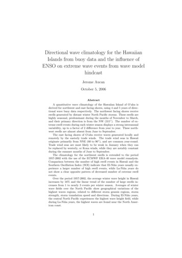
The wave heights and directions show little change between deep water andthe buoy locations (figure 2). For Waimea buoy, the change in incidence angleα due to refraction is less than 1 for waves of 17 s period or less. The change inwave height due to shoaling is less than 2 % for waves of 17 s period or less. ForMokapu buoy, the change in incidence angle from deep water wave conditionsdue to refraction is less than 1 for waves of 15 s period or less. The changein wave height due to shoaling is less than 4 % for waves of 15 s period or less(figure 2).The process of wave diffraction operates in regions where refraction createsa gradient of wave height along the direction perpendicular to the wave ray, oralong the wave crest. Diffraction transmits energy from area of high energy toareas of low energy. In our case, refraction is minimal, so the effect of diffractionat the buoy locations is considered negligible.2.32.3.1Northwest swells at Waimea BuoyDirectional climatologyWe first investigate the general characteristics of the incoming northwest swells.The directional spectrum at the Waimea buoy is averaged over each availablemonth (figure 3). Due to the position of the Waimea buoy relative to theisland of O’ahu, we only use the Waimea buoy to investigate the northwestswells originating between the W and NNE directions. The northwest swells arepredominant during the months of October to March (figure 3), with a maximumin January. Their direction is predominantly from the NW (315 , figure 3), andthe associated period between 10 and 20 s. At the location of Waimea buoy, theshore normal direction is approximately 300 relative to true North. Accordingto figure 2, the predominant swells measured at the buoy ( 300 to 330 ,10 to 20 s) underwent a change in wave height and a change of incidence anglebelow 5% and 1 respectively compared to their deep water characteristics. Weconsequently conclude that the average directional wave climate measured atthe Waimea buoy is representative of an open ocean location offshore of Hawaii,unobstructed for waves originating from the 300 to 25 relative to truenorth. The island of Kauai blocks swells that originate from directions around290 . It is unclear to what extent the decrease of energy south of the 300 sectoris due to the presence of the island or due to the storm paths in the North Pacificfavoring waves in Hawaii coming from the 315 sector. Since 2005, the NationalData Buoy Center upgraded station 51001, located 170 nm West Northwest ofKauai Island, to a directional wave buoy. In the future, data from this buoy,coupled with a local wave modelling effort, could quantify the two effects.A second energy peak is clearly visible year-round in the NE quadrant, andis associated with the trade wind swells and seas. The Waimea buoy is notcompletely sheltered from the trade wind swells by the island of Oahu, butthese swells and seas have undergone significant directional change (20 to 40 )by the time they are measured by the buoy. The trade wind swell and seas willbe discussed in more details in the following section using the Mokapu buoy.5
In January, there is also noticeable energy in the SW to NW quadrant, atlower period (5 to 10 s, figure 3), that is associated with locally generated seasfrom the SW to NW direction (Kona Winds conditions).2.3.2Extreme events distributionTo investigate the distribution of swell heights on the northwest facing shores, wecalculate the wave height corresponding to this particular directional quadrant.In this section we focus on the NW quadrant at Waimea buoy, and calculateHsigN W by integrating the directional spectrum S(θ, ω) over the W to NNEquadrant, for all available frequencies.sZ θ 22.5 Z ω 0.58 HzHsigN W 4S(θ, ω)dθdω(8)θ 270 ω 0.025 HzFor consistency with the wave models sampling intervals, we use a 3-hour average of S(θ, ω) to calculate HsigN W .For each month, we calculate the mean wave height, and the percentagedistribution of given wave heights (figure 4). The highest average wave heightoccurs in January, when HsigN W 2.4 m. In January HsigN W 3 m, 25% ofthe time and HsigN W 1 m only 5% of the time. In sharp contrast, the lowestaverage HsigN W occur in July when HsigN W 0.5 m and HsigN W 1 m,more than 95% of the time.A typical year can be divided in 4 seasons (Figure 4). The winter season(November to March), when the occurrence of high swell event ( 3 m) is high, 2transitional seasons (April, May and October), when moderate swells (1 to 3 m)are common, and a low season when waves are typically 1 m in June, July,August and September. In terms of the shoreline definition, it is obvious that thehighest reach of the waves should be estimated during the period of Novemberto March.2.42.4.1Trade winds swell and seas from Mokapu BuoyDirectional climatologyThe Mokapu buoy is used to investigate the climatology of the trade windsswell and seas, that originate from the SE to NNE directions. The trade windsea directional spectrum shows a predominant energy peak between 6 and 12 speriods and 60 to 90 direction relative to true north, all year-round (figure5). Compared to the northwest swells, this pattern shows less variations frommonth to month during the period observed (2001-2005). The northwest swellsdescribed in the previous section are also clearly visible at Mokapu buoy, butundergo significant refraction, and will not be discussed here any further. Athird peak of energy is visible in the average for the month of November (figure5), at long periods ( 20 s), from the NNE. This is due to one extremely highevent in November 2003, that caused damages to houses, beach closures andflooded roadways. According to local elders, this had not been seen since 506
years. This swell was not higher than the other high swell originating from thenorthwest, but its direction made it a very unusual event in Hawaii.2.4.2Events distributionWe now focus on the east quadrant at Mokapu buoy. We calculate HsigEby integrating the 3-hourly averages directional spectrum S(θ, ω) over the Equadrant:sZ θ 135 Z ω 0.58 HzHsigE 4S(θ, ω)dθdω(9)θ 22.5 ω 0.025 HzIn January, the average wave height HsigE from the trade wind seas is thesmallest ( 1 m, figure 6). In January, the trades can also be absent for longperiods of time, as they are replaced by westerly (or Kona) winds. Over theobserved period, the wave height in January for the trade wind seas is 1 m 56%of the time. During the summer, from June to September, trade wind seas arevery constant, with 1 HsigE 2 m, over 75% of the time (figure 6), with amaximum in July (90% of the time).33.1Interannual variability of extreme events inHawaiiWave model reanalysisThe timeserie of buoy data in Hawaii (5 years) is too short to investigate theinterannual variability of extreme events in the context of large scale climateindices. To extend the time series of wave height in Hawaii, two different wavemodel reanalyses are used. Both model are based on the WAM wave model([7]), use the same basic physics, but different wind forcing products.The National Centers for Environmental Prediction of the National Oceanicand atmospheric Administration (NCEP/NOAA) provides a global historicalwave model on a 1.25 latitude 1 longitude grid. This model is called theNOAA WaveWatch III or WW3 ([8]). Historical reanalysis data are availableevery 3 hours from January 30 1997.The European Center for Medium-range Weather Forecasting (ECMWF)produced a global wave reanalysis (ERA-40,[9]) on a 1.5 latitude 1.5 longitudegrid, for the period 1957-2002. The wave model was forced by hourly winds,and output was available every 6-hours.For each model, the significant wave height Hsig, peak wave period Tp andpeak wave direction Dp are extrapolated from the global wave fields at eachtime step, at a point north of Oahu, Hawaii (figure 1, 22 N, 158 W ). WW3archive does not include time series of directional spectrum, and no funding wasavailable at the time to obtain time series of directional spectrum near Hawaiifrom the ERA-40 reanalysis. Therefore, directional climatologies from the wave7
models similar to the ones obtained from buoy data on figures 5 and 3 are notpossible at this time.3.2Extreme eventsIt is apparent on figures 5 and 3 that the directional wave spectrum in Hawaiiduring the winter is usually bimodal, with one peak at low-frequency from thenorthwest, and one peak at high frequency from the east. Significant waveheights Hsig from the wave models are calculated with all frequencies anddirections. If no swell other than the northwest swell and the trade wind sea ispresent in the area, then by definition22Hsig 2 HsigNW HsigE(10)2During extreme winter events however, the contribution of HsigEto Hsig is222small (HsigN W À HsigE ), so we can compare HsigN W from the buoy, to Hsigfrom the model reanalysis. To prevent identification of south swells or easterlyswells, we only keep the Hsig from the model reanalysis when the correspondingpeak wave direction Dp satisfies Dp 25 or Dp 270 . To identify anindividual swell, we use the daily average of wave height from the buoy andthe model and identify local maxima. For each winter season, the number oflarge swell events (Hsig 4 m) is calculated from the two models and theWaimea Buoy (figure 7). Over the period 1997-2001, the two models producesthe same number of extreme events (to within 1 event). Over the period 20012004, when model and buoy data overlap, there are larger differences betweenthe numbers of events produced by the model or the buoy timeserie (figure 7).The differences can be due to inherent errors in the wave models, or relatedthe different methods for calculating wave height. When available, this analysisshould be redone using the directional spectrum time series from the ERA40 reanalysis. Nonetheless, we will use the extreme events statistics from theERA-40 wave model in the following section.3.3Long term trend and relation to climate indicesTo estimate the influence of El-Niño, we calculate the average Southern Oscillation Index (SOI) for each winter season (November to March), and comparewith the number of large events in Hawaii from the ERA-40 model, and theWW3 model (figure 8). The SOI climate index was obtained from the NationalOceanic and Atmospheric Administration/ Cooperative Institute for Researchin Environmental Sciences (NOAA/CIRES) Climate Diagnostic Center (CDC).The Southern Oscillation Index (SOI) is defined as the normalized pressure difference between Tahiti and Darwin. There are several slight variations in theSOI values calculated at various centres. Here we use the SOI from the ClimateResearch Unit (CRU) at the University of East Anglia, which is based on themethod given by [10]. A negative SOI indicates an El-Niño event, while a positive SOI indicates a La Niña event. Here, we arbitrarily define El-Niño eventswhen the winter average of SOI is SOI 1, and Niña event when SOI 0.5.8
We extend the calculation of extreme events (Hsig 4 m) to the 1957-2002period, using the timeserie of wave height produced by the ERA-40 reanalysis(figure 8). The number of extreme events for each winter season (NovemberMarch) varies significantly from year to year, from 7 events during the strongEl-Niño period of 1997-1998, to no events at all. The number of extreme eventsfrom the ERA-40 reanalysis shows a significant increasing linear trend over theperiod 1957-2002 (figure 8), from just over 1 major event per season in 1958to over 3 events per season in 2001. Over the period 1957-2002, the significantwave height averaged for each winter season (November to March) shows a 16%increase. This is consistent with the intensification of North Pacific Winter Cyclones ([3] and others). If we add the period 2002-2005 (figure 7), the increasingtrend will likely be even more pronounced. During all El-Niño events (65-66,7778,82-83,86-87,91-92,97-98), Hawaii experience more extreme events than theaverage trend (figure 8). La-Niña years do not necessarily coincide with lessextreme events.An increase of the number of high swell events over the same period wasalso documented in California ([4]). This increase may be related to the averagewave field in the North Pacific. We use our arbitrary threshold for defining SOIstate (figure 8) to produce winter averages (November-March) of wave heightfrom the ERA-40 reanalysis over the North Pacific, for the two extreme SOIconditions (figure 9 top and and bottom), and for the overall average (figure9 middle). The wave heights averaged over the winters of strong El-Niño arehigher than the average (figure 9). Differences in wave height reach up to 1 m inthe central North Pacific between El-Niño years average and the overall average.Differences in wave height between the La-Niña years average and the overallaverage are not as large.The time-averaged wave height field shows different geographical distribution(figure 9) during El-Niño or La-Niña years. The overall average for the 1957-2002period (figure 9 middle) shows two areas of increased wave height, the first inthe central North Pacific, centered around 40 N and 175 W , and a second oneoffshore of North America, near 45 N and 135 W . During El-Niño years (figure9 top), the central Pacific high wave area is predominant, and no secondarymaximum in wave height is observed near the North American coast. DuringLa-Niña years (figure 9 bottom), the North American coast region experiencesthe highest time-averaged wave heights.The wave heights are not only related to the wind speed during a storm,but also to the storm translation speed and direction ([11]). The differencesin the geographical distribution of high wave height between El-Niño and LaNiña years indicate differences in the combination of cyclogenesis regions andstorms intensities and trajectories. A more in-depth description of the physicalmechanisms explaining these differences is out of the scope of this paper.9
4Summary and discussionWe have described the wave climate for the northwest and east facing shoresof the Island Of Oahu, Hawaii, with data from 2 different buoys (figures 3 to6). This wave climatology quantifies the average wave energy received by eachshore, and will be useful for the studies of biological and physical processeswhere wave play an active role. A direct comparison of this measurementbased directional wave climatology with the results of two widely used wavemodel products (WaveWatch III and ERA-40) was not possible because of theunavailability of directional spectrum time-serie from the models.We use the results from the wave models to extend the northwest extremeevents climatology to the period 1957-2002 (figure 8). We found that the numberof extreme events (larger than 4 m) increased over the period, and that duringEl-Niño years, Hawaii experiences a larger number of extreme events. Mapsof time-averaged wave height in the North Pacific also show higher basin-widewave heights during El-Niño years. The geographical distribution of high waveheights is different during El-Niño and La-Niña years (figure 9), and is likelyrelated to a combination of different cyclogenesis regions and different stormsintensities and trajectoriesAcknowledgmentsThe directional waverider buoys used in this study were purchased through aDURIP grant from the Office of Naval Research. Funding for the maintenanceof the buoys, and the salary of the author were provided by Dr. Mark Merrifield, director of the University of Hawaii Sea-Level-Center (UHSLC), throughthe Joint Institute of Marine and Atmospheric Research (JIMAR). The staffat the Coastal Data Information Program (CDIP), and Julie Thomas in particular, provided invaluable technical advice and were responsible for the dataacquisition and archiving of the buoys. ERA-40 data was retrieved from theonline catalog of the European Center for Medium-Range Weather Forecasts(ECMWF).References[1] R. W. Grigg. Holocene coral reef accretion in hawaii: A function of waveexposure and sea level history. Coral Reef, 17:263–272, 1998.[2] D. K. Woolf, P. G. Challenor, and P. D. Cotton. Variability and predictability of the North Atlantic wave climate. Journal of Geophysical Research(Oceans), 107:9–1, October 2002.[3] N.E. Graham and H.F. Diaz. Evidence for intensification of north pacificwinter cyclones since 1948. bams, 2001.10
[4] R. Seymour. Wave climate variability in southern california. J. Wtrwy.,Port, Coast., and Oc. Engrg., 122(4):182–186, 1996.[5] A. Lygre and H. Krogstad. Maximum entropy estimation of the directionaldistribution in ocean wave spectra. J. Phys. Oceanogr., 16:2052–2060, 1986.[6] R. B. Long. The statistical evaluation of directional spectrum estimatesderived from pitch/roll buoy data. J. Phys. Oceanogr., 1980.[7] WAMDI. The wam model-a third generation ocean wave prediction model.J. Phys. Oceanogr., 18:1775–1810, 1988.[8] H. L. Tolman. User manual and system documentation of wavewatch-iiiversion 1.18. Technical report, Ocean Modeling Branch, NCEP, NationalWeather Service, NOAA, Department of Commerce, 1999.[9] S. Caires, A. Sterl, J.R. Bidlot, N. Graham, and V. Swail. Intercomparisonof different wind-wave reanalyses. J. Climate, 17:1893–1913, 2004.[10] C.F. Ropelewski and P.D. Jones. An extension of the Tahiti-Darwin southern oscillation index. Month. Weath. Rev., 115:2161–2165, 1987.[11] J. Wolf and D.K. Woolf. Waves and climate change in the north-eastAtlantic. Geophys. Res. Letters, 00%Aug30%100%100%100%93%100%Table 1: Mokapu Point buoy availability, in 0%100%100%100%100%100%
100%Sep0%0%80%0%100%100%Table 2: Waimea Bay buoy availability, in percentFigure 1: Top : Location map of the Hawaiian Islands chain, and wave modelouput (red triangle). Bottom : Bathymetry of Oah’u and location of the waverider buoys (red 00%Dec0%51%100%100%100%100%
Mokapu Point BuoyWaimea Bay Buoy4545 520 4 3201510105505101520025 1 1 21525 2incidence angle (o)o2530 3incidence angle ( )35 6 530 435 140 9 8 7 4 3 2 1405Wave period .980300.92incidence angle (o)0.9205250.940.960.98o35188incidence angle ( )0.0.920.940.960.982510200.90.92453015Wave period (s)4535105025Wave period (s)510152025Wave period (s)Figure 2: Effect of refraction between deep water and the depth at the buoylocation for Mokapu Point buoy (left) and Waimea Bay buoy (right). Change ofangle of incidence (degree) as a function of deep water incidence angle and waveperiod (top), and refraction and and shoaling coefficient (Kr Ks ) as a functionof deep water incidence angle and wave period (bottom)13
JanFeb25 13 86AprMar25 13 86May25 13 86Jul25 13 86Oct625 13 86625 138625 138625 1386Sep6Nov25 13 88JunAug25 13 825 13Dec25 13 86Figure 3: Averages of directional spectra for each months at Waimea Bay buoy.color scale is logarithmic, constant over all frames, and covers 2 orders of magnitude. Values that are a factor 3 smaller than the maximim are not plotted. Redlines show the sector of the origin of waves used for the calculation of HsigN W14
JanFebHsig 2.36 / 1.1m80Hsig 1.77 / 6033Hsig 2.01 / 0.91m804022DecHsig 1.61 / 0.83m806011NovHsig 1.21 / 0.69m805%404460%%6033Hsig 0.702 / 0.26m804022SepHsig 0.531 / 0.21m806011AugHsig 0.572 / 0.16m805%404460%%6033Hsig 0.631 / 0.25m804022JunHsig 0.872 / 0.36m806011MayHsig 1.13 / 0.53m80Hsig 1.79 / 0.81m8060%60Mar12345012345Figure 4: Histograms of occurrence (in percent of time) of wave height HsigN Wfor each months at Waimea buoy. Blue bars indicate the mean for each monthwhen calculated over all the available years, and red bars indicate minima andmaxima for each month and wave size. Mean wave height is indicated for eachmonth plus or mi
2.1 Data collection and measurement principle Mokapu Point buoy was first deployed August 9 2000, offshore of Kailua Bay on the windward side of O'ahu, in 120 m water depth. Data from this buoy is archived by the Coastal Data Information Program (CDIP) as station CDIP 098, and by the National Data Buoy Center as station NDBC 51202. Waimea