Transcription
The Pricing of Tail Risk and the Equity Premium:Evidence from International Option Markets Torben G. Andersen† Nicola Fusari‡ Viktor Todorov§August 2018AbstractWe explore the pricing of tail risk as manifest in index options across international equity markets. The risk premium associated with negative tail events displays persistent shifts, unrelatedto volatility. This tail risk premium is a potent predictor of future returns for all the indices,while the option-implied volatility only forecasts the future return variation. Hence, compensation for negative jump risk is the primary driver of the equity premium, whereas the reward forpure diffusive variance risk is unrelated to future equity returns. We also document pronouncedcommonalities, suggesting a high degree of integration among the major global equity markets.Keywords: Equity Risk Premium, International Option Markets, Predictability, Tail Risk,Variance Risk Premium.JEL classification: G12, G13, G15, G17. Andersen gratefully acknowledges support from CREATES, Center for Research in Econometric Analysis of TimeSeries (DNRF78), funded by the Danish National Research Foundation. The work is partially supported by NSF GrantSES-1530748. We thank the Editor, Todd Clark, the Associate Editor, and two anonymous referees for many usefulcomments and suggestions. We thank Eben Lazarus for providing the code used to implement the HAR estimatorsin Lazarus et al. (2018). We also thank participants at the following presentations for useful comments: AQR CapitalManagement; Midwest Finance Association Meeting 2016, Chicago; Key-note address at the 2016 Nippon FinanceAssociation Meeting, Yokohama; 30th Anniversary of GARCH Models and Measures Conference, Toulouse School ofEconomics; Key-note address at the Financial Econometrics and Empirical Asset Pricing Conference 2016, LancasterUniversity Management School; SoFiE Annual Meeting 2016, City University, Hong Kong; NBER Summer Institute2016; Financial Econometrics Conference 2016, Questrom School of Business, Boston University; CBOE Conferenceon Volatility and Derivatives 2016, Chicago; Financial Econometrics Conference 2016, Rio de Janeiro; as well asparticipants at numerous seminars.†Kellogg School, Northwestern University, Evanston, IL 60208, email: t-andersen@northwestern.edu.‡The Johns Hopkins University Carey Business School, Baltimore, MD 21202, email: nfusari1@jhu.edu.§Kellogg School, Northwestern University, Evanston, IL 60208, email: v-todorov@northwestern.edu.
1IntroductionOver the last decade, global financial markets have been roiled by major shocks, including thefinancial crisis originating in October 2008 and European debt crises in May 2010 and August2011. These events represent a challenge to dynamic asset pricing models. Can they accommodatethe observed interdependencies between volatility and tail events, and their pricing? How dovolatility and tails differ across countries? How do the variance and tail risk premiums relate tothe compensation for exposure to equity risk, i.e., the equity premium? The increasing liquidityof derivative markets worldwide provides an opportunity to shed light on these questions. Inparticular, the trading of equity-index options has grown sharply, with both more strikes permaturity and additional maturities on offer. Most importantly, there has been a dramatic increasein the trading of options with short tenor. As a result, we now have access to active prices forsecurities that embed rich information about the pricing of volatility and tail risk in many separatecountries. By combining the pricing of financial risks, embodied within the equity-index optionsurfaces, with ex-post information on realized returns, volatilities and jumps, we can gauge therelative size of the risk premiums and what factors drive the risk compensation.In the current work, we draw on daily observations for option indices in the U.S. (S&P 500),Euro-zone (ESTOXX), Germany (DAX), Switzerland (SMI), U.K. (FTSE), Italy (MIB), and Spain(IBEX) over 2007-2014 to extract factors that are critical for the pricing of equity market risk acrossNorth America and Europe. The performance of the individual equity indices varies drastically, withthe German market appreciating by an average of about 8% per year and the Italian depreciatingby 5% annually, as illustrated in Figure 1. This heterogeneity provides additional power in studyingthe connection between market tail risk and the equity risk premium.Most existing option pricing models capture the dynamics of the equity-index option surfacethrough the evolution of factors that determine the volatility of the underlying stock market, see,e.g., Bates (1996, 2000, 2003), Pan (2002), Eraker (2004) and Broadie et al. (2007). However,recent evidence suggests that the fluctuations in the left tail of the risk-neutral density, extractedfrom equity-index options, can be spanned neither by regular volatility factors nor by realizedrisk measures constructed from return data. Hence, a distinct factor is necessary to account forthe priced downside risk in the option surface, see Andersen et al. (2015b). We accommodatesuch features by specifying a parametric risk-neutral return model, but imposing no structural1
Cumulative 15Figure 1: Country-specific cumulative equity-index cum dividend log-returns. The sourceof the data used in constructing the figure are detailed in Section ?.assumptions on the underlying return generating process. Other models allowing for an element ofseparation between jump and volatility factors include Santa-Clara and Yan (2010), Christoffersenet al. (2012), Gruber et al. (2015), and Li and Zinna (2018).We seek to fully exploit the available information by utilizing all option quotes that satisfyour mild filtering criteria. This is important because the European samples are short and displayvarying liquidity. Such features render day-by-day factor identification more challenging than forthe U.S. market. Consequently, we specify a parsimonious risk-neutral model with a single volatilitycomponent along with the tail factor. The short-dated options are highly informative regardingthe current level of volatility and jump intensities, while the longer-dated options primarily speakto the factor dynamics. In combination, this facilitates robust identification of the volatility andjump components and reduces the number of parameters in the risk-neutral model, providing asolid basis for out-of-sample exploration of the predictive power of the option-implied factors.We briefly summarize our empirical findings. Most importantly, we find a substantial discrepancy between the time series evolution of priced tail risk and volatility for every option market weanalyze. A common feature emerges in the aftermath of crises – the left tail factor is correlatedwith volatility, yet it remains elevated long after volatility subsides to pre-crisis levels. This isincompatible with the usual approach to the modeling of volatility and jump risk in the literature.The stark separation of the tail and volatility factors has important implications for the pricing2
and dynamics of market risk. Even though volatility is a strong predictor of future market risk, itprovides no forecast power for the equity risk premium. In contrast, our left tail factor does not helppredict future market risks, yet it has highly significant explanatory power for future market returns.The tail factor also constitutes the primary driver of the negative tail risk premium, suggesting thisis the operative channel through which it forecasts the equity premium. In particular, followingcrises, equity prices are heavily discounted and the option-implied tail factor remains elevated, evenas market volatility resides. Throughout our sample, this combination serves a strong signal thatthe market will outperform in the future.These findings inspire a number of new, interrelated hypotheses regarding the relative forecastpower of option-implied and return variation measures for the equity risk premium, which wevalidate for each of our equity indices. For example, the compensation for exposure to returnvariation, i.e., the variance risk premium or VRP, has been intensely studied following the workof Carr and Wu (2009) and Bollerslev et al. (2009). We find, most strikingly, that the VRP onlyforecasts future equity returns because it embeds the left tail factor. Once the jump risk premium isstripped from the VRP, it no longer provides a signal for the performance of the equity market. Sincethe VRP constructed from different asset classes also have predictive power for the correspondingexcess returns, e.g., credit spreads (Wang et al. (2013)), currency returns (Londono and Zhou(2017)), and bond returns (Mueller et al. (2017)), our results likely have broader implications forrisk pricing across diverse global security markets.In terms of the volatility factor, we find the European and U.S. markets to evolve in near unisonthrough the financial crisis of 2008-2009. In contrast, we observe discrepancies during and afterthe initial European sovereign debt crisis. Overall, the U.K., Swiss and, to some extent, Germanvolatilities remain close throughout the sample. The largest divergences in volatility dynamicsoccur between the U.S., U.K. and Swiss (non euro-zone) indices on one side and the Spanish andItalian on the other, with the latter representing the Southern euro-zone countries in our sample.For the left tail factor, there are interesting commonalities and telling differences. Again, themain discrepancies are associated with the Southern European indices. Specifically, the Spanishtail factor reacts strongly to both phases of the sovereign debt crisis, while the Italian response ismore muted, especially for the first phase.Exploiting the extracted factor realizations along with estimates for the risk-neutral and actual3
return dynamics, we further document very strong dependence between the negative jump riskpremiums for the equity indices throughout the sample. By contrast, the dependence between thediffusive risk premiums across markets is strong only for the financial crisis period 2007-2009, whilefor 2010-2014, associated with the European sovereign debt crises, the dependence between thediffusive risk premiums weakens significantly. Given the critical role of the tail factor for futureequity returns, the coherence in the compensation for tail risk across indices rationalizes the strongcorrelation of the drift component among the individual equity indices, evident in Figure 1, despitethe heterogeneity in the severity of the shocks affecting the individual countries.Our work is related to an evolving literature on the ability of equity option and equity returnvariation measures to capture the pricing of exposure to volatility and tail, jump or skew risk. Byextension, such measures should possess forecast power for future equity returns. First, there is oldliterature studying empirically the mean variance tradeoff and the ability of stock market volatilityto predict future returns, see e.g., French et al. (1987) and Glosten et al. (1993) for early references.More recently, Almeida et al. (2017), Bali et al. (2009) and Kelly and Jiang (2014) use differentapproaches to construct tail measures from the cross-section of observed stock prices and show thatthese measures can predict future market returns.The above cited work does not use derivatives in the construction of the tail and volatility measures. Employing individual equity options, Bali and Hovakimian (2009) find that both the variancerisk premium and an alternative option spread measure—interpreted as a jump risk measure—explain cross-sectional variation in expected returns. Later, Conrad et al. (2013) find that morenegative risk-neutral volatility and skew measures are associated with higher returns in the crosssection. The latter is consistent with the evidence of preferences for positive skew equity assetsobtained in Bali and Murray (2013).For the U.S. equity index, Bollerslev and Todorov (2011) document that a nonparametricbased left tail premium measure explains a significant fraction of both the variance and equityrisk premium. Bollerslev et al. (2015) and Du and Kapadia (2012) show that nonparametric jumptail measures constructed from options can predict returns in the future over horizons of severalmonths, while Atilgan et al. (2013) find evidence for short-term return predictability (daily andweekly) by option-implied measures. Meanwhile, Kozhan et al. (2013) demonstrate that the skewrisk premium is substantial, but overlaps with the variance risk premium, and conclude that these4
risk factors have a common source. Finally, Li and Zinna (2018) find that both the level and slopeof the term structure for the variance risk premium provide significant predictors of future equityreturns.On the international front, Bollerslev et al. (2014) show that local VRPs provide qualitativelysimilar, yet decidedly weaker, predictive power for national equity-index returns than in the U.S.However, a weighted average of the VRP measures provides a global proxy with significantly improved explanatory power across the indices. Similarly, Londono (2016) find that foreign VRPmeasures are insignificant predictors for the local equity returns, but the U.S. VRP provide muchsuperior performance, with only the Japanese index remaining unpredictable. Finally, Gao et al.(2018) establish predictive power for the excess returns on a wide set of asset classes using a globaltail index, constructed in accordance with the “jump and tail” index of Du and Kapadia (2012).Our findings are consistent with existing results in many respects. The VRP has predictivepower for equity returns, but negative tail measures perform even better; the pricing of equity riskhas a strong global component; and equity-index returns are highly correlated across countries.Yet, our contribution deviates from the prior literature on numerous points. Most importantly,we identify a component in the risk-neutral left jump intensity, orthogonal to spot volatility, whichwe show is the main driver of the equity return predictability. Raw option-implied risk measures(volatility or tail related) have weaker predictive ability, rationalizing some of the existing empiricalresults in the literature. Our findings suggest the existence of an important wedge between riskand risk premium dynamics for all the equity indices in our analysis.Two, in contrast to most prior studies, we exploit the information across all option maturitiesand strikes. Earlier work typically relies on one maturity only and aggregate many options into asingle measure, such as the volatility level or skew. Our use of short-dated options enhances ourability to identify the current state of the volatility and jump factors. Moreover, the observationsfor the longer tenors facilitate identification of the risk-neutral volatility and jump dynamics.Three, we decompose the variance risk premium into a number of separate elements and providea strict rank ordering of their ability to forecast equity-index returns. In particular, the continuousreturn variation and associated premium should have no predictive power. These new hypothesesare corroborated for each of the equity indices.Four, we obtain strong empirical results for return predictability based on the foreign option5
panels. The U.S. evidence remains highly significant, but not more so than for many of the othercountries. This finding is consistent with our approach affording an improved extraction of information from the smaller sample of options available outside the U.S.Finally, the only existing work we are aware of linking tail measures with equity return predictability internationally is Gao et al. (2018). Their tail index captures the variation in the higherorder risk-neutral moments induced by jumps, which is controlled by the variation in the jump intensity. In contrast to our left tail factor, the tail index of Gao et al. (2018) covaries quite stronglywith volatility. Moreover, by construction, their index puts most of the weight on very deep outof-the-money option prices. This may render the tail measure somewhat unstable, as the activestrike coverage is subject to fluctuations in liquidity and the contracts are subject to relatively largemeasurement errors. By contrast, we are less sensitive to liquidity and data availability issues, butat the cost of imposing some parametric structure on the option dynamics.The paper is organized as follows. Section 2 presents the model used to fit the option surfaces,and Section 3 reviews the estimation method. Section 4 focuses on the option-implied factors andtheir predictive ability. Section 5 explores the interaction among the factors and the risk premiums,with emphasis on the role of the jump factor. We study the common features in the option-impliedfactors and risk premiums in Section 6. Finally, Section 7 concludes. Additional details on data,estimation method and results are provided in the online Appendix.2ModelThis section introduces our model for the risk-neutral dynamics of a generic equity market index,denoted X, and defines a set of related risk measures and premiums explored in the empirical work.The model is designed to capture the dynamics of the option surface through a low-dimensionalstate vector within a continuous-time no-arbitrage setting. We subsequently use the option-impliedstate vector to predict future equity risks and risk premiums and relate these to sources of pricedrisk in the economy. Because the European option samples are limited relative to the U.S., we seeka robust and parsimonious specification that captures the salient features and facilitates a sharpday-by-day separation of the volatility and jump factors. Towards that end, we are inspired byprior successful representations, but limit ourselves to one volatility and one jump intensity factor.6
2.1The Risk-Neutral Equity-Index DynamicsOur two-factor model for the risk-neutral index dynamics is given by the following restricted versionof the representation in Andersen et al. (2015b),ZpdXt (rt δt ) dt Vt dWtQ (ex 1) µeQ (dt, dx) ,Xt RZpQdVt κv (v Vt ) dt σv Vt dBt µvx2 1{x 0} µ(dt, dx) ,RZdUt κu Ut dt µux2 1{x 0} µ(dt, dx) ,(1)Rwhere(WtQ , BtQ ) is a two-dimensional Brownian motion with corr WtQ , BtQ ρ, while µ denotesan integer-valued measure counting the jumps in the index, X, as well as the state vector, (V, U ),representing the spot variance and negative jump intensity. We denote the corresponding jumpcompensator by dt νtQ (dx), so the difference, µeQ (dt, dx) µ(dt, dx) dt νtQ (dx), constitutes theassociated martingale jump measure. Finally, the drift term equals the risk-free interest rate minusthe (continuous) dividend payout ratio, ensuring that the expected instantaneous return (underthe risk-neutral measure) of the cum-dividend price process equals the risk-free rate.The jump component, x, captures price jumps, but also scenarios involving co-jumps. Specifically, for negative price jumps of size x, the two state variables, V and U , display (positive) jumpsproportional to x2 . Thus, the jumps in the spot variance and negative jump intensity are co-linear,albeit with distinct proportionality factors, µv and µu . This specification involves a substantialamplification from the negative price shocks to the risk factors. The compensator characterizes theconditional jump distribution and takes the form,νtQ (dx) λ x Ut · 1{x 0} λ e λ x c .0 · 1{x 0} λ edx(2)Following Kou (2002), we assume that the price jumps are exponential, with separate taildecay parameters, λ and λ , for negative and positive jumps. Finally, the left jump intensityis governed by the factor Ut while the positive jump intensity is constant and equal to c 0 . Thelatter assumption is innocuous. We verify that all qualitative empirical conclusions are robust tostandard specifications of time variation in the positive jump factor.Our jump modeling includes novel features and deviates markedly from the standard parametricspecification in the empirical option pricing literature. First, the price jumps are exponentiallydistributed, and consequently have fat tails, while most prior studies rely on Gaussian price jumps,7
following Merton (1976). Second, the jumps in the factors V and U are linked deterministicallyto the negative price jumps, with the squared jumps impacting the factor dynamics in a mannerreminiscent of discrete GARCH models. Third, and most importantly for the analysis here, thejump intensity is time-varying, and with innovations that are linked directly to the volatility andprice jumps, yet its dynamics is largely decoupled from volatility. This is unlike most existingmodels, with the notable exception of Christoffersen et al. (2012), Gruber et al. (2015) and Li andZinna (2018). Nonetheless, the representation (1) belongs to the affine class of models of Duffieet al. (2000).1 For future reference, we label our two-factor affine model the 2F U model.The model is motivated by recent evidence that the negative jump intensity represents a separaterisk factor which is essential in capturing the dynamics in the left side of the option surface.Moreover, that study finds the left tail factor to be a critical driver of the variation in the equity andvariance risk premiums. At the same time, model (1) provides a more parsimonious representationthan the preferred specification in Andersen et al. (2015b), which features two separate volatilityfactors. This choice reflects our desire to achieve precise identification of the relevant jump factorfrom the shorter, less liquid option samples encountered in this study. As discussed in Section 4below, the jump factor is robustly identified in the current more restricted model.2.2Risk Measures and Risk PremiumsWe conclude the section by introducing a few risk measures and associated risk premiums that areused throughout the paper. The quadratic variation of the log-price is given by,Zt hσs2 dsZt h Zx2 µ(ds, dx). tt(3)RWe denote its conditional risk-neutral expectation by QVt,t h ,QVt,t h CVt,t h JVt,t h EtQ"Zt h#Vt dt tEtQ"Zt h#Zxt2νtQ (dx),(4)Rwhere CVt,t h and JVt,t h are the expected diffusive and jump variation under the risk-neutralmeasure, respectively.2 The expected jump variation JVt,t h , can be decomposed further into1There is some option-based evidence, see, e.g., Jones (2003) and Christoffersen et al. (2010), that non-affinemodels work better. The fact that our key findings are driven primarily by short-maturity options should mitigatethe importance of potential misspecification stemming from nonlinearities in the volatility dynamics.2For notational simplicity, we often do not include a superscript Q to indicate that a specific quantity is obtainedunder the risk-neutral measure. For example, the expected diffusive return variation under the risk-neutral measure8
terms stemming from negative and positive jumps,JVt,t h N JVt,t h P JVt,t h EtQ Zt h Ztx 0 Z x2 νtQ (dx) EtQtt h Zx 0 x2 νtQ (dx) .Importantly, N JVt,t h is proportional to Ut , while its level, of course, is tied also to the jumpsize distribution. Specifically, for the 2F U model, the instantaneous risk-neutral negative jumpvariation N JVt (i.e., with h 0) equals,ZN JVt x2 νtQ (dx) x 02Ut .λ2 (5)In contrast, the (risk-neutral) expected positive jump variation, P JVt,t h , is constant and equals2c 0 λ2 h. Finally, due to the jumps in Vt , CVt,t h is, in general, an affine function of both Vt and Ut . However, we document later that, empirically, almost all variation in CVt,t h stems from Vt .The above measures can also be computed under the equivalent statistical measure (P), whichleads to the definition of the variance risk premium as,PV RPt,t h QVt,t h QVt,t h,and the negative jump risk premium as,PN JRPt,t h N JVt,t h N JVt,t h.Our computation of the expected return variation measures under the statistical (P) measurefollows standard high-frequency procedures for forecasting the volatility and jump risks. That is,we do not specify a parametric model for X under P. Instead, we use a reduced-form model togenerate the necessary conditional P-expectations for the calculation of the requisite risk premiums,exploiting the popular HAR model of Corsi (2009). Consistent with our empirical evidence inSection 4.2.1 below, we find only lagged continuous return variation measures, and not laggedjump variation measures, to be significant predictors of the future return variation. Appendix A.3provides a detailed description of these procedures.Qis denoted CVt,t h rather than CVt,t h. This should not cause confusion as, whenever we refer to expectations underthe actual or statistical probability measure, the relevant quantities carry the superscript P.9
3Estimation ProcedureWe follow the inference procedures in Andersen et al. (2015a) for recovering the parameters andlatent factor realizations of model (1). The option prices are converted into Black-Scholes impliedvolatilities (BSIV), i.e., any out-of-the-money (OTM) option price observed at time t with tenor τand log moneyness k log (K/Ft,t τ ) is represented by the BSIV, κt,k,τ . For a given state vector,St (Vt , Ut ), and parameter vector θ, the model-implied BSIV is denoted κk,τ (St , θ). Estimationnow proceeds by minimizing the distance between observed and model-implied BSIV in a metricthat also penalizes for discrepancies between the inferred spot volatilities and those estimated (inqa model-free way) from high-frequency data on the underlying asset, Vbtn , see Appendix A.3 forfurther details. The imposition of (statistical) equality between the spot volatility estimated fromthe actual and risk-neutral measure reflects a basic no-arbitrage condition implied by the underlyingoption pricing paradigm.To formally specify the estimation criterion, we introduce additional notation. Let t 1, . . . , T ,denote the dates for which we observe the option prices at the end of trading. We focus on OTMoptions, with k 0 indicating OTM puts and k 0 OTM calls. Due to put-call parity and thelower liquidity of in-the-money options, there is little loss of information from using only OTMoptions for estimation.We obtain point estimates for the risk-neutral parameter vector θ and period-by-period statevector St (Vt , Ut ) from the following optimization problem, see Andersen et al. (2015a), 2T XXκt,kj ,τj κkj ,τj (St , θ)0.05Tb t } , θb argmin{S t 1NNtt{St }T ,θ t 1t 1τj ,kjq 2 Vbtn VtVbtn /2.(6)To reduce the computational burden, we estimate the system for options only sampled on Wednesday or, if this date is missing, the following trading day. Credible identification of the system isobtained by observing heterogeneous constellations of the option surface across time. We facilitatethis objective by exploiting all, including very short-dated, options that satisfy a mild filter, designed to identify whether a given option observation is flawed. The surface varies dramatically forthe early and late years relative to the periods around the financial and European debt crises. Oncethe parameter vector and the state variable realizations for all Wednesdays have been obtained,it is straightforward to “filter” the state variables for the remaining trading days, exploiting the10
estimated parameters, option data, and the criterion (6). Thus, we obtain daily estimates for thestate realizations, even if full-fledged estimation is performed only for weekly data.We emphasize that the estimation procedure is devoid of parametric assumptions concerningthe underlying equity-index returns. We only impose the no-arbitrage condition that implies equality between the spot volatility under the risk-neutral and objective measure, while allowing for(statistical) deviations that reflect measurement errors for both the option pricing model impliedvolatility estimator and the nonparametric high-frequency return based spot volatility estimator.4Option FactorsThe data used for our empirical analysis of the U.S., Eurozone, German, British, Swiss, Italian,and Spanish equity indices are described in Appendix A.1. As discussed in Section 2, our modelis restricted relative to Andersen et al. (2015b). We confirm, however, that the analysis is robustto a more refined modeling of the volatility dynamics by documenting near identical jump factorextraction from the alternative models in Appendix A.5. Additional details on our estimationresults are provided in Appendix A.6.4.1Country-by-Country Factor RealizationsThis section explores the implied factor realizations obtained from model (1) and the estimationprocedure outlined in Section 3. We first compare the spot variance of the European indices,benchmarking against the S&P 500 results.Figure 2 plots the extracted volatilities from the ESTOXX (Eurozone), DAX (Germany), SMI(Switzerland), FTSE 100 (U.K.), MIB (Italy), and IBEX 35 (Spain) markets. We note the extraordinary close association between many of these factors and the S&P 500 spot volatility, not justin terms of correlation, but also level. For example, the U.K. volatility is barely distinguishablefrom the S&P 500 factor throughout, while the Swiss factor deviates visibly from the S&P 500 onlyduring a few episodes after the Swiss franc-euro exchange rate cap imposed in September 2011. Inthe former case, the volatility correlation is about 98% and in the latter 95%.In contrast, notable discrepancies between the S&P 500 and German DAX emerge during thesecond phase of the European sovereign debt crisis, when the DAX volatility spikes more, and apositive gap remains from that point onward, albeit to a varying degree. For the broader ESTOXX11
index, the same effect is clear
Evidence from International Option Markets Torben G. AndersenyNicola Fusariz Viktor Todorovx August 2018 Abstract We explore the pricing of tail risk as manifest in index options across international equity mar-kets. The risk premium associated with negative tail events displays persistent shifts, unrelated to volatility.