Transcription
SAS/OR 15.1 User’s GuideMathematical ProgrammingThe NonlinearProgramming Solver
This document is an individual chapter from SAS/OR 15.1 User’s Guide: Mathematical Programming.The correct bibliographic citation for this manual is as follows: SAS Institute Inc. 2018. SAS/OR 15.1 User’s Guide: MathematicalProgramming. Cary, NC: SAS Institute Inc.SAS/OR 15.1 User’s Guide: Mathematical ProgrammingCopyright 2018, SAS Institute Inc., Cary, NC, USAAll Rights Reserved. Produced in the United States of America.For a hard-copy book: No part of this publication may be reproduced, stored in a retrieval system, or transmitted, in any form or byany means, electronic, mechanical, photocopying, or otherwise, without the prior written permission of the publisher, SAS InstituteInc.For a web download or e-book: Your use of this publication shall be governed by the terms established by the vendor at the timeyou acquire this publication.The scanning, uploading, and distribution of this book via the Internet or any other means without the permission of the publisher isillegal and punishable by law. Please purchase only authorized electronic editions and do not participate in or encourage electronicpiracy of copyrighted materials. Your support of others’ rights is appreciated.U.S. Government License Rights; Restricted Rights: The Software and its documentation is commercial computer softwaredeveloped at private expense and is provided with RESTRICTED RIGHTS to the United States Government. Use, duplication, ordisclosure of the Software by the United States Government is subject to the license terms of this Agreement pursuant to, asapplicable, FAR 12.212, DFAR 227.7202-1(a), DFAR 227.7202-3(a), and DFAR 227.7202-4, and, to the extent required under U.S.federal law, the minimum restricted rights as set out in FAR 52.227-19 (DEC 2007). If FAR 52.227-19 is applicable, this provisionserves as notice under clause (c) thereof and no other notice is required to be affixed to the Software or documentation. TheGovernment’s rights in Software and documentation shall be only those set forth in this Agreement.SAS Institute Inc., SAS Campus Drive, Cary, NC 27513-2414November 2018SAS and all other SAS Institute Inc. product or service names are registered trademarks or trademarks of SAS Institute Inc. in theUSA and other countries. indicates USA registration.Other brand and product names are trademarks of their respective companies.SAS software may be provided with certain third-party software, including but not limited to open-source software, which islicensed under its applicable third-party software license agreement. For license information about third-party software distributedwith SAS software, refer to http://support.sas.com/thirdpartylicenses.
Chapter 11The Nonlinear Programming SolverContentsOverview: NLP Solver . . . . . . . . . . . . . . . . . . . . . . . . . . . . . . . . . . . . .531Getting Started: NLP Solver . . . . . . . . . . . . . . . . . . . . . . . . . . . . . . . . . .533Syntax: NLP Solver . . . . . . . . . . . . . . . . . . . . . . . . . . . . . . . . . . . . . . .545Functional Summary . . . . . . . . . . . . . . . . . . . . . . . . . . . . . . . . . . .545NLP Solver Options . . . . . . . . . . . . . . . . . . . . . . . . . . . . . . . . . . .546Details: NLP Solver . . . . . . . . . . . . . . . . . . . . . . . . . . . . . . . . . . . . . .Basic Definitions and Notation . . . . . . . . . . . . . . . . . . . . . . . . . . . . .553553Constrained Optimization . . . . . . . . . . . . . . . . . . . . . . . . . . . . . . . .554Interior Point Algorithm . . . . . . . . . . . . . . . . . . . . . . . . . . . . . . . . .555Interior Point Direct Algorithm . . . . . . . . . . . . . . . . . . . . . . . . . . . . .557Active-Set Method . . . . . . . . . . . . . . . . . . . . . . . . . . . . . . . . . . . .559Multistart . . . . . . . . . . . . . . . . . . . . . . . . . . . . . . . . . . . . . . . . .561Covariance Matrix . . . . . . . . . . . . . . . . . . . . . . . . . . . . . . . . . . . .562Iteration Log for the Local Solver . . . . . . . . . . . . . . . . . . . . . . . . . . . .565Iteration Log for Multistart . . . . . . . . . . . . . . . . . . . . . . . . . . . . . . .565Solver Termination Criterion . . . . . . . . . . . . . . . . . . . . . . . . . . . . . . .566Solver Termination Messages . . . . . . . . . . . . . . . . . . . . . . . . . . . . . .567Macro Variable OROPTMODEL . . . . . . . . . . . . . . . . . . . . . . . . . . .567Examples: NLP Solver . . . . . . . . . . . . . . . . . . . . . . . . . . . . . . . . . . . . .570Example 11.1: Solving Highly Nonlinear Optimization Problems . . . . . . . . . . .570Example 11.2: Solving Unconstrained and Bound-Constrained Optimization Problems572Example 11.3: Solving Equality-Constrained Problems . . . . . . . . . . . . . . . . .574Example 11.4: Solving NLP Problems with Range Constraints . . . . . . . . . . . . .576Example 11.5: Solving Large-Scale NLP Problems . . . . . . . . . . . . . . . . . . .579Example 11.6: Solving NLP Problems That Have Several Local Minima . . . . . . .581Example 11.7: Maximum Likelihood Weibull Estimation . . . . . . . . . . . . . . . .587Example 11.8: Finding an Irreducible Infeasible Set . . . . . . . . . . . . . . . . . .589References . . . . . . . . . . . . . . . . . . . . . . . . . . . . . . . . . . . . . . . . . . .594Overview: NLP SolverThe sparse nonlinear programming (NLP) solver is a component of the OPTMODEL procedure that can solveoptimization problems containing both nonlinear equality and inequality constraints. The general nonlinear
532 F Chapter 11: The Nonlinear Programming Solveroptimization problem can be defined asminimize f .x/subject to hi .x/ D 0; i 2 E D f1; 2; : : : ; pggi .x/ 0; i 2 I D f1; 2; : : : ; qgl x uwhere x 2 Rn is the vector of the decision variables; f W Rn 7! R is the objective function; h W Rn 7! Rpis the vector of equality constraints—that is, h D .h1 ; : : : ; hp /; g W Rn 7! Rq is the vector of inequalityconstraints—that is, g D .g1 ; : : : ; gq /; and l; u 2 Rn are the vectors of the lower and upper bounds,respectively, on the decision variables.It is assumed that the functions f; hi , and gi are twice continuously differentiable. Any point that satisfiesthe constraints of the NLP problem is called a feasible point, and the set of all those points forms the feasibleregion of the NLP problem—that is, F D fx 2 Rn W h.x/ D 0; g.x/ 0; l x ug.The NLP problem can have a unique minimum or many different minima, depending on the type of functionsinvolved. If the objective function is convex, the equality constraint functions are linear, and the inequalityconstraint functions are concave, then the NLP problem is called a convex program and has a unique minimum.All other types of NLP problems are called nonconvex and can contain more than one minimum, usuallycalled local minima. The solution that achieves the lowest objective value of all local minima is called theglobal minimum or global solution of the NLP problem. The NLP solver can find the unique minimum ofconvex programs and a local minimum of a general NLP problem. In addition, the solver is equipped withspecific options that enable it to locate the global minimum or a good approximation of it, for those problemsthat contain many local minima.The NLP solver implements the following primal-dual methods for finding a local minimum: interior point trust-region line-search algorithm interior point line-search algorithm, which uses direct linear algebra active-set trust-region line-search algorithmThese three methods can solve small-, medium-, and large-scale optimization problems efficiently androbustly, and they use exact first and second derivatives to calculate search directions. The memory requirements of all algorithms are reduced dramatically because only nonzero elements of matrices are stored.Convergence of all algorithms is achieved either (1) by using a trust-region line-search framework that guidesthe iterations toward the optimal solution or (2) by simply performing a backtracking line search. For the firstconvergence technique, if a trust-region subproblem fails to provide a suitable step of improvement, a linesearch is then used to fine-tune the trust-region radius and ensure sufficient decrease in objective functionand constraint violations. The second convergence technique is a backtracking line search on a primal-dualmerit function.The NLP solver implements two primal-dual interior point algorithms. Both methods use barrier functions toensure that the algorithm remains feasible with respect to the bound constraints. Interior point methods areextremely useful when the optimization problem contains many inequality constraints and you suspect thatmost of these constraints will be satisfied as strict inequalities at the optimal solution.The active-set technique implements an active-set algorithm in which only the inequality constraints thatare satisfied as equalities, together with the original equality constraints, are considered. Once that set of
Getting Started: NLP Solver F 533constraints is identified, active-set algorithms typically converge faster than interior point algorithms. Theyconverge faster because the size and the complexity of the original optimization problem can be reduced ifonly few constraints need to be considered.For optimization problems that contain many local optima, the NLP solver can be run in multistart mode. Ifthe multistart mode is specified, the solver samples the feasible region and generates a number of startingpoints. Then the local solvers can be called from each of those starting points to converge to different localoptima. The local minimum with the smallest objective value is then reported back to the user as the optimalsolution.The NLP solver implements many powerful features that are obtained from recent research in the field ofnonlinear optimization algorithms (Akrotirianakis and Rustem 2005; Armand, Gilbert, and Jan-Jégou 2002;Armand and Omheni 2017a, b; Erway, Gill, and Griffin 2007; Forsgren and Gill 1998; Vanderbei 1999;Wächter and Biegler 2006; Yamashita 1998). The term primal-dual means that the algorithm iterativelygenerates better approximations of the decision variables x (usually called primal variables) in addition to thedual variables (also referred to as Lagrange multipliers). At every iteration, the algorithm uses a modifiedNewton’s method to solve a system of nonlinear equations. The modifications made to Newton’s method areimplicitly controlled by the current trust-region radius. The solution of that system provides the direction andthe steps along which the next approximation of the local minimum is searched. The active-set algorithmensures that the primal iterations are always within their bounds—that is, l x k u, for every iteration k.However, the interior approach relaxes this condition by using slack variables, and intermediate iterationsmight be infeasible.Finally, for parameter estimation problems such as least squares, maximum likelihood, or Bayesian estimationproblems, the NLP solver can calculate the covariance matrix after it successfully obtains parameter estimates.Getting Started: NLP SolverThe NLP solver consists of three techniques that can solve a wide class of optimization problems efficientlyand robustly. This section presents three examples that introduce the three techniques of NLP. The examplesalso introduce basic features of the modeling language of PROC OPTMODEL that is used to define theoptimization problem.The NLP solver can be invoked using the SOLVE statement,SOLVE WITH NLP / options ;where options specify the technique name, termination criteria, and how to display the results in the iterationlog. For a detailed description of the options, see the section “NLP Solver Options” on page 546.A Simple ProblemConsider the following simple example of a nonlinear optimization problem:minimize f .x/ D .x1 C 3x2 C x3 /2 C 4.x1subject to x1 C x2 C x3 D 16x2 C 4x3 x13 3 0xi 0; i D 1; 2; 3x2 /2
534 F Chapter 11: The Nonlinear Programming SolverThe problem consists of a quadratic objective function, a linear equality constraint, and a nonlinear inequalityconstraint. The goal is to find a local minimum, starting from the point x 0 D .0:1; 0:7; 0:2/. You can use thefollowing call to PROC OPTMODEL to find a local minimum:proc optmodel;var x{1.3} 0;minimize f (x[1] 3*x[2] x[3])**2 4*(x[1] - x[2])**2;con constr1: sum{i in 1.3}x[i] 1;con constr2: 6*x[2] 4*x[3] - x[1]**3 - 3 0;/* starting point */x[1] 0.1;x[2] 0.7;x[3] 0.2;solve with NLP;print x;quit;Because no options have been specified, the default solver (INTERIORPOINT) is used to solve the problem.The SAS output displays a detailed summary of the problem along with the status of the solver at termination,the total number of iterations required, and the value of the objective function at the best feasible solutionthat was found. The summaries and the returned solution are shown in Figure 11.1.Figure 11.1 Problem Summary, Solution Summary, and the Returned SolutionThe OPTMODEL ProcedureProblem SummaryObjective SenseObjective FunctionObjective TypeMinimizationfQuadraticNumber of Variables3Bounded Above0Bounded Below3Bounded Below and Above0Free0Fixed0Number of Constraints2Linear LE ( )0Linear EQ ( )1Linear GE ( )0Linear Range0Nonlinear LE ( )0Nonlinear EQ ( )0Nonlinear GE ( )1Nonlinear Range0
Getting Started: NLP Solver F 535Figure 11.1 continuedSolution SummarySolverNLPAlgorithmInterior PointObjective FunctionfSolution StatusBest FeasibleObjective Value1.0000158715Optimality ns5Presolve Time0.00Solution 0The SAS log shown in Figure 11.2 displays a brief summary of the problem being solved, followed by theiterations that are generated by the solver.Figure 11.2 Progress of the Algorithm as Shown in the LogNOTE: Problem generation will use 16 threads.NOTE: The problem has 3 variables (0 free, 0 fixed).NOTE: The problem has 1 linear constraints (0 LE, 1 EQ, 0 GE, 0 range).NOTE: The problem has 3 linear constraint coefficients.NOTE: The problem has 1 nonlinear constraints (0 LE, 0 EQ, 1 GE, 0 range).NOTE: The OPTMODEL presolver removed 0 variables, 0 linear constraints, and 0nonlinear constraints.NOTE: Using analytic derivatives for objective.NOTE: Using analytic derivatives for nonlinear constraints.NOTE: The NLP solver is called.NOTE: The Interior Point algorithm is 7251.000017380.00000002508830.0000005000000NOTE: Optimal.NOTE: Objective 1.000017384.NOTE: Objective of the best feasible solution found 1.0000158715.NOTE: The best feasible solution found is returned.NOTE: To return the local optimal solution found, set the SOLTYPE option to 0.
536 F Chapter 11: The Nonlinear Programming SolverA Least Squares ProblemAlthough the NLP solver does not implement techniques that are specialized for least squares problems,this example illustrates how the NLP solver can solve least squares problems by using general nonlinearoptimization techniques.The Bard function, f .x/, (Moré, Garbow, and Hillstrom 1981) is a least squares problem with n D 3parameters and m D 15 functions fi :15f .x/ D1X 2fi .x/;2x D .x1 ; x2 ; x3 /i D1where the functions are defined as uifi .x/ D yix1 Cvi x2 C wi x3with ui D i , vi D 16i, wi D min.ui ; vi /, andy D .0:14; 0:18; 0:22; 0:25; 0:29; 0:32; 0:35; 0:39; 0:37; 0:58; 0:73; 0:96; 1:34; 2:10; 4:39/Starting from x 0 D .1; 1; 1/, you can reach the minimum at the point .0:08; 1:13; 2:34/, with correspondingobjective value f .x / 4.107E–3. You can use the following SAS code to formulate and solve this problem:proc optmodel;set S 1.15;number u{i in S} i;number v{i in S} 16 - i;number w{i in S} min(u[i], v[i]);number y{S} [ .14 .18 .22 .25 .29 .32 .35 .39 .37 .58.73 .96 1.34 2.10 4.39 ];var x{1.3} init 1;min f 0.5 * sum{i in S} ( y[i] ( x[1] u[i]/(v[i] * x[2] w[i] * x[3]) )) 2;solve with nlp / algorithm ipdirect;print x;quit;The output that summarizes the problem characteristics and the solution that the IPDIRECT solver obtainsare displayed in Figure 11.3.
Getting Started: NLP Solver F 537Figure 11.3 Problem Summary, Solution Summary, and Returned SolutionThe OPTMODEL ProcedureProblem SummaryObjective SenseMinimizationObjective FunctionfObjective TypeNonlinearNumber of Variables3Bounded Above0Bounded Below0Bounded Below and Above0Free3Fixed0Number of Constraints0Solution SummarySolverNLPAlgorithmInterior Point DirectObjective FunctionfSolution StatusOptimalObjective Value0.0041074387Optimality Error3.1901663E-8Infeasibility0Iterations7Presolve Time0.00Solution Time0.00[1]x10.08241121.13303632.343696The SAS log shown in Figure 11.4 displays a brief summary of the problem being solved, followed by theiterations that are generated by the solver.
538 F Chapter 11: The Nonlinear Programming SolverFigure 11.4 Progress of the Algorithm as Shown in the LogNOTE: Problem generation will use 16 threads.NOTE: The problem has 3 variables (3 free, 0 fixed).NOTE: The problem has 0 linear constraints (0 LE, 0 EQ, 0 GE, 0 range).NOTE: The problem has 0 nonlinear constraints (0 LE, 0 EQ, 0 GE, 0 range).NOTE: The OPTMODEL presolver removed 0 variables, 0 linear constraints, and 0nonlinear constraints.NOTE: Using analytic derivatives for objective.NOTE: The NLP solver is called.NOTE: The experimental Interior Point Direct algorithm is 002289770.0041074400.0000000319017NOTE: Optimal.NOTE: Objective 0.0041074387.A Larger Optimization ProblemConsider the following larger optimization problem:P1 P52minimize f .x/ D 1000j D1 zjiD1 xi yi C 2P5subject to xk C yk C j D1 zj D 5; for k D 1; 2; : : : ; 1000P1000P5i D1 .xi C yi / Cj D1 zj 61 xi 1; i D 1; 2; : : : ; 10001 yi 1; i D 1; 2; : : : ; 10000 zi 2; i D 1; 2; : : : ; 5The problem consists of a quadratic objective function, 1,000 linear equality constraints, and a linearinequality constraint. There are also 2,005 variables. The goal is to find a local minimum by using theACTIVESET technique. This can be accomplished by issuing the following call to PROC OPTMODEL:proc optmodel;number n 1000;number b 5;var x{1.n} -1 1 init 0.99;var y{1.n} -1 1 init -0.99;var z{1.b} 0 2 init 0.5;minimize f sum {i in 1.n} x[i] * y[i] sum {j in 1.b} 0.5 * z[j] 2;con cons1{k in 1.n}: x[k] y[k] sum {j in 1.b} z[j] b;con cons2: sum {i in 1.n} (x[i] y[i]) sum {j in 1.b} z[j] b 1;
Getting Started: NLP Solver F 539solve with NLP / algorithm activeset logfreq 10;quit;The SAS output displays a detailed summary of the problem along with the status of the solver at termination,the total number of iterations required, and the value of the objective function at the local minimum. Thesummaries are shown in Figure 11.5.Figure 11.5 Problem Summary and Solution SummaryThe OPTMODEL ProcedureProblem SummaryObjective SenseMinimizationObjective FunctionfObjective TypeQuadraticNumber of Variables2005Bounded Above0Bounded Below0Bounded Below and Above2005Free0Fixed0Number of Constraints1001Linear LE ( )0Linear EQ ( )1000Linear GE ( )1Linear Range0Solution SummarySolverAlgorithmObjective FunctionNLPActive SetfSolution StatusOptimalObjective Value-996.4999999Optimality 0Presolve Time0.00Solution Time0.18The SAS log shown in Figure 11.6 displays a brief summary of the problem that is being solved, followed bythe iterations that are generated by the solver.
540 F Chapter 11: The Nonlinear Programming SolverFigure 11.6 Progress of the Algorithm as Shown in the LogNOTE: Problem generation will use 16 threads.NOTE: The problem has 2005 variables (0 free, 0 fixed).NOTE: The problem has 1001 linear constraints (0 LE, 1000 EQ, 1 GE, 0 range).NOTE: The problem has 9005 linear constraint coefficients.NOTE: The problem has 0 nonlinear constraints (0 LE, 0 EQ, 0 GE, 0 range).NOTE: The OPTMODEL presolver removed 0 variables, 0 linear constraints, and 0nonlinear constraints.NOTE: Using analytic derivatives for objective.NOTE: Using 2 threads for nonlinear evaluation.NOTE: The NLP solver is called.NOTE: The Active Set algorithm is 0.00000000883120.0000003954618NOTE: Optimal.NOTE: Objective -996.4999999.An Optimization Problem with Many Local MinimaConsider the following optimization problem:minimize f .x/ D e sin.50x/ C sin.60e y / C sin.70 sin.x// C sin.sin.80y//sin.10.x C y// C .x 2 C y 2 / 4subject to1 x 11 y 1The objective function is highly nonlinear and contains many local minima. The NLP solver provides youwith the option of searching the feasible region and identifying local minima of better quality. This isachieved by writing the following SAS program:proc optmodel;var x -1 1;var y -1 1;min f exp(sin(50*x)) sin(60*exp(y)) sin(70*sin(x)) sin(sin(80*y))- sin(10*(x y)) (x 2 y 2)/4;solve with nlp / multistart (maxstarts 30) seed 94245;quit;The MULTISTART () option is specified, which directs the algorithm to start the local solver from manydifferent starting points. The SAS log is shown in Figure 11.7.
Getting Started: NLP Solver F 541Figure 11.7 Progress of the Algorithm as Shown in the LogNOTE: Problem generation will use 16 threads.NOTE: The problem has 2 variables (0 free, 0 fixed).NOTE: The problem has 0 linear constraints (0 LE, 0 EQ, 0 GE, 0 range).NOTE: The problem has 0 nonlinear constraints (0 LE, 0 EQ, 0 GE, 0 range).NOTE: The OPTMODEL presolver removed 0 variables, 0 linear constraints, and 0nonlinear constraints.NOTE: Using analytic derivatives for objective.NOTE: The NLP solver is called.NOTE: The Interior Point algorithm is used.NOTE: The MULTISTART option is enabled.NOTE: The deterministic parallel mode is enabled.NOTE: The Multistart algorithm is executing in single-machine mode.NOTE: The Multistart algorithm is using up to 16 threads.NOTE: Random number seed 94245 is timal30-3.3068686-3.30686865E-704OptimalNOTE: The Multistart algorithm generated 640 sample points.NOTE: 30 distinct local optima were found.NOTE: The best objective value found by local solver -3.306868647.
542 F Chapter 11: The Nonlinear Programming SolverFigure 11.7 continuedNOTE: The solution found by local solver with objective -3.306868647 wasreturned.The SAS log presents additional information when the MULTISTART () option is specified. The first columncounts the number of restarts of the local solver. The second column records the best local optimum thathas been found so far, and the third through sixth columns record the local optimum to which the solver hasconverged. The final column records the status of the local solver at every iteration.The SAS output is shown in Figure 11.8.Figure 11.8 Problem Summary and Solution SummaryThe OPTMODEL ProcedureProblem SummaryObjective SenseMinimizationObjective FunctionfObjective TypeNonlinearNumber of Variables2Bounded Above0Bounded Below0Bounded Below and Above2Free0Fixed0Number of Constraints0Solution SummarySolverAlgorithmObjective FunctionMultistart NLPInterior PointfSolution StatusOptimalObjective Value-3.306868647Number of Starts30Number of Sample Points640Number of Distinct Optima30Random Seed UsedOptimality ErrorInfeasibility942455E-70Presolve Time0.00Solution Time0.06
Getting Started: NLP Solver F 543A Least Squares Estimation Problem for a Regression ModelThe following data are used to build a regression model:data samples;input x1 x2 y;datalines;4 843.7162 5 351.2981 62 2878.9185 75 3591.5965 54 2058.7196 84 4487.8798 29 1773.5236 33 767.5730 91 1637.663 59 215.2862 57 2067.4211 48 394.1166 21 932.8468 24 1069.2195 30 1770.7834 14 368.5186 81 3902.2737 49 1115.6746 80 2136.9287 72 3537.84;Suppose you want to compute the parameters in your regression model based on the preceding data, and themodel isL.a; b; c/ D a x1 C b x2 C c x1 x2where a; b; c are the parameters that need to be found.The following PROC OPTMODEL call specifies the least squares problem for the regression model:/* Reqression model with interactive term: y a*x1 b*x2 c*x1*x2 */proc optmodel;set obs;num x1{obs}, x2{obs}, y{obs};num mycov{i in 1. nvar , j in 1.i};var a, b, c;read data samples into obs [ n ] x1 x2 y;impvar Err{i in obs} y[i] - (a*x1[i] b*x2[i] c*x1[i]*x2[i]);min f sum{i in obs} Err[i] 2;solve with nlp/covest (cov 5 covout mycov);print mycov;print a b c;quit;The solution is displayed in Figure 11.9.
544 F Chapter 11: The Nonlinear Programming SolverFigure 11.9 Least Squares Problem Estimation ResultsThe OPTMODEL ProcedureProblem SummaryObjective SenseMinimizationObjective FunctionfObjective TypeQuadraticNumber of Variables3Bounded Above0Bounded Below0Bounded Below and Above0Free3Fixed0Number of Constraints0Solution SummarySolverNLPAlgorithmInterior PointObjective FunctionfSolution StatusOptimalObjective Value7.1862967833Optimality e Time0.00Solution Time0.01mycov1231 0.00000478252 -.0000000996 0.00000324263 -.0000000676 -.0000000442 0.0000000017abc3.0113 2.0033 0.4998
Syntax: NLP Solver F 545Syntax: NLP SolverThe following PROC OPTMODEL statement is available for the NLP solver:SOLVE WITH NLP / options ;Functional SummaryTable 11.1 summarizes the options that can be used with the SOLVE WITH NLP statement.Table 11.1 Options for the NLP SolverDescriptionCovariance Matrix Options and SuboptionsRequests that the NLP solver compute a covariancematrixSpecifies an absolute singularity criterion for matrixinversionSpecifies the type of covariance matrixSpecifies the name of the output covariance matrixSpecifies the tolerance for deciding whether a matrix issingularSpecifies a relative singularity criterion for matrix inversionSpecifies a number for calculating the divisor for thecovariance matrix when VARDEF DFSpecifies a number for calculating the scale factor for thecovariance matrixSpecifies a scalar factor for computing the covariance matrixSpecifies the divisor for calculating the covariance matrixMiscellaneous OptionSpecifies the seed to use to generate random numbersMultistart OptionsDirects the local solver to start from multiple initial pointsSpecifies the maximum range of values that each variablecan take during the sampling processSpecifies the tolerance for local optima to be considereddistinctSpecifies the amount of printing solution progress inmultistart modeSpecifies the time limit in multistart modeSpecifies the maximum number of starting points to beused by the multistart algorithmOptimization OptionSpecifies the optimization techniqueOptionCOVEST ()ASINGULAR COV COVOUT COVSING MSINGULAR NDF NTERMS SIGSQ VARDEF SEED MULTISTART ()BNDRANGE DISTTOL LOGLEVEL MAXTIME MAXSTARTS ALGORITHM
546 F Chapter 11: The Nonlinear Programming SolverTable 11.1 Options for the NLP Solver (continued)DescriptionOutput OptionsSpecifies the frequency of printing solution progress (localsolvers)Specifies the allowable types of output solutionSolver OptionsSpecifies the feasibility toleranceSpecifies the type of Hessian used by the solverEnables or disables IIS detection with respect to linear constraints and variable boundsSpecifies the maximum number of iterationsSpecifies the time limit for the optimization processSpecifies the upper limit on the objectiveSpecifies the convergence toleranceSpecifies whether the solver is allowed to shift the user-suppliedinitial point to be interior to the boundsSpecifies units of CPU time or real timeOptionLOGFREQ SOLTYPE FEASTOL HESSTYPE IIS MAXITER MAXTIME OBJLIMIT OPTTOL PRESERVEINIT TIMETYPE NLP Solver OptionsThis section describes the options that are recognized by the NLP solver. These options can be specifiedafter a forward slash (/) in the SOLVE statement, provided that the NLP solver is explicitly specified using aWITH clause.Covariance Matrix OptionsCOVEST (suboptions)requests that the NLP solver produce a covariance matrix. When this option is applied, the followingPROC OPTMODEL options are automatically set: PRESOLVER NONE and SOLTYPE 0. For moreinformation, see the section “Covariance Matrix” on page 562.You can specify the following suboptions:ASINGULAR asingspecifies an absolute singularity criterion for measuring the singularity of the Hessian andcrossproduct Jacobian and t
global minimum or global solution of the NLP problem. The NLP solver can find the unique minimum of convex programs and a local minimum of a general NLP problem. In addition, the solver is equipped with specific options that enable it to locate the global minimum or a good approximation of it, for those problems that contain many local minima.