WIXLIB

can be exercised at any moment between purchase and expiration, whereas the lattercan be exercised only at expiration. They were called “privileges” because theygranted buyers the right (privilege) of choosing to exercise them or not.Moreover, those options investors from the very beginning seem to have beenrather sophisticated. If we used today’s Black-Scholes model to analyze the skewpremium (the higher price for out-of-the-money options versus at-the-money options)on US shares, we’d see that they anticipated the banking crisis of 1873 six monthsbefore its onset.2By the early 20th century, options markets were sufficiently developed in theUS and throughout Europe that arbitrage trading by telegraph became possiblebetween New York and London. Besides stock options, the FX options market beganoperating in the mid-19th century and was active at the beginning of the 20th century.3That activity stimulated interest in a specialized options literature. Castelli in1877 described put-call parity, Higgins in 1902 and Nelson in 1904 explained deltahedging. Haug and Taleb believe that the first formulas for option calculations werepublished by Vinzenz Bronzin in 1908. In 1967, Van Thorpe and Kassouf offered amathematical formula that systematized dynamic hedging principles. By applying hisfindings Van Thorpe became one of history’s most successful hedge fund managers,beating the S&P during most of his 20 years managing money. 4 Contrary to commonbelief, as Haug and Taleb and others point out, options markets were operatingsoundly before the 1970s—i.e., before invention of the Black-Scholes model.5Today’s Black-Scholes formula, now known to most market participants, isessentially a more elegant presentation of long-previously developed concepts. It is,however, its elegance that allowed the contemporary options market to expand andbecome one of the more powerful financial markets today.10

Put / Call Parity and Its ApplicationsPut / Call ParityPut / call parity (formerly called the option arbitrage formula) is thefoundation of options theory and position management. It also has a lengthy history.Known from the late 19th century, it was mentioned by L.R. Higgins in The Putand-Call published in London in 1902 and by S.A. Nelson in The ABC of Optionsand Arbitrage published in New York in 1904.6Both refer to earlier books, including The Theory of Options by Charles Castelli in1877,7 so this principle may have been known then. The concept is the basis ofmodern options theory because it balances all market components and does not allowmispricing of combinations of options and their underlying assets (in today’sunderstanding cash / spot / futures / forwards) with similar economic and riskprofiles.To explain the formula we need to recap the basic facts of options trading. Onthe day of expiration, an option will either expire or get exercised. If a call isexercised, its owner will buy the underlying asset at the option strike price. Then hecan sell that asset, receiving its current market price that is higher than the strikeprice. If a put is exercised, its owner will sell the underlying asset at the option strikeprice and will be able to buy it, paying its market price that is lower than the strikeprice8. These logical sequences are expressed by the put / call parity formula, asimplified form of which is:Parity (Pricecall Priceput) (Price at Expirationunderlying asset Option Strike Price).9Let’s demonstrate how the formula works using a simple example with Applestock option. Let's say you own one 600 Apple call and the 600 put in equalamounts. By options exchange rules, each stock option is exercisable into 100shares. If the stock trades at 610 on the day of expiration, the call can beexercised—i.e., you can buy the stock at 600 per share and sell it for 610, gaining 1,000 (100 shares x 10 per share). Instead of exercising the call, you can sell it for 1,000. The corresponding put in this situation expires worthless.If at expiration the stock trades at 590, you can sell the stock at 600 per shareand buy it for 590, or you can sell the put for 1,000, Therefore, the put is worth 1,000, while the call is worthless.11

Let’s apply this logic to the formula. On the day of expiration, the prices of thecall and the put will equal the difference between each option’s strike price and theprice of the underlying asset. When the call and the put have equal strike prices, atexpiration your gain on one means the loss on the other. As a separate case, if atexpiration the stock trades at 600, both the call and the put expire worthless, while(Price at Expirationunderlying asset Option Strike Price) is equal 0. Please note that ifyou buy the call and the put simultaneously, you have a chance to profit if the stockmoves either direction.Now, let's try a variation that forms the basis of modern options theory and isdescribed in its many explanatory books. What if you buy two 600 Apple calls andsell short 100 shares of Apple instead of buying one call and one put, as in theexample above?x If on expiration day the stock trades at 610, the call will be worth 2,000 (2 x 10 x 100), while the position in shares will lose 1,000 ( 10 x 100). In totalyou will make 1000.x If on expiration the stock trades at 590, the call will expire worthless, whereasthe short sale will earn you 1,000 ( 10 x 100). In total, you earn 1,000.What if you buy two 600 Apple puts and buy 100 shares of Apple?x If on expiration the stock trades at 590, the put will be worth 2,000 (2 x 10x 100), while the position in shares will lose 1000. In total, you earn 1000.x If on expiration the stock trades at 610, the put will expire worthless, whilethe position in shares will earn 1,000. In total, you earn 1,000.In all three cases the results of similar moves up and down are the samenotwithstanding the difference in positions. Especially interesting are the latter twoexamples, where the position based on the call gives the same result as the positionbased on the put. If there is no difference in their economic performance—i.e., theyprovide similar benefit—would you agree that their price should be the same? Hencethere should be parity between the prices you pay for both positions.12

Two Important RemarksSimple adjustments to the logic above, which we’ll discuss in later chapters,show that put / call parity works not only at expiration, but any time prior.In the market vernacular, the options in the second and third examples were“hedged with the underlying.” As you saw, the performance of the hedged positionsin our examples was the same when the underlying asset moved in either direction.This observation leads to an interesting and crucial detail: options pricing modelsassume an equal probability that prices of the underlying asset could rise or fall. Thatis, they ignore directional forecasts of the underlying asset’s price! In other words,prices of a call and a put with the same strike price and expiration date should beidentical. This is a very foreign concept for those who trade the underlying positionswhich by nature are directional. We will expand on this concept in the next chapter.Applying the Option Arbitrage (Put / Call Parity) Formula to Determine the TwoComponents of an Option Premium’s Intrinsic Value and Time ValueAn option premium consists of intrinsic value and time value. Assuming youcan exercise a purchased option at any time at a profit, the gain you’d earn is calledthe option’s intrinsic value. In the examples, above if on expiration of one 600 callthe stock trades at 610 then its intrinsic value was 1,000 (1 x 10 x 100). Besidesintrinsic value, option prices contain time value—that part of the option’s price thatreflects the worth implicit in how long you control the right to buy or sell theunderlying asset. In fact, the idea behind options is essentially to gain ownership oftime value. If there is none, the option in economic terms doesn’t exist!As shown above, the potential gain of both hedged calls and hedged puts withthe same strikes and expiration dates is the same. Hence their time values should beidentical. It’s up to you whether you hedge, but since the theory assumes you will,their time value should be equal. This is not to say that their premiums will be equal.For example, if the current share price of Apple is 610 and the price of one 600Apple call expiring in three months is 1,800, the call’s intrinsic value is 1,000 (1 x( 610 600) x 100). Its time value is 800 ( 1,800 1,000). Therefore, the timevalue of the 600 Apple put is also 800. Because this put is out of the money, itsintrinsic value is 0.If the price of Apple is 592 and the price of one 600 put is 1,500, the put’sintrinsic value is 800 (1 x ( 600 592) x 100). The time value is 1500 800 13

700. Therefore, the time value of the equivalent 600 call also would be 700.Since this call is out of the money, its intrinsic value is 0.MoneynessInvestors also refer to options by the relation of their strike price to the currentprice of the underlying security, called moneyness. That is, they say an option isATM (at the money), ITM (in the money), and OTM (out of the money). Options withintrinsic value are called ITM. Options whose strike price equals the current price ofthe underlying are called ATM. Finally, options which have no intrinsic value andare not ATM are called OTM. We will use those abbreviations throughout theremainder of the book.Hedge Ratio, DeltaEarlier we noted that option hedging has existed since late 19th century. Backthen, dealers realized that options with different strikes required different quantitiesof the underlying hedge. The relationship of the amount of hedge to the amount ofthe option was called the hedge ratio. It was equal to the probability of an exercisethat the dealer attributed to a given option. Nowadays we call the hedge ratio delta,and we calculate it using Black-Scholes or other options formulas.Delta shows sensitivity of the option premium to the changes of the value ofthe underlying value. To give a practical example, if you own a call on shares of aparticular company, a delta of 0.50 means that for every 1 increase in the price ofthe underlying stock, the option’s price—its premium—rises 0.50. In practice, thedecimal point is ignored; the delta is said to be 50, and the option is said to be 50delta. ATM options are 50-delta. Delta of ITM options exceeds 50%, and delta ofOTM options is less than 50. A deep OTM option, i.e. an option with delta close to100, will change in value at the same rate as the underlying.Application of Put / Call Parity for Building Synthetic PositionsThe relationship of put and call prices established by put / call parity permitstraders to combine options and forwards to create synthetic positions. Parity also wasthe basis for the claim that the time value of calls and puts with the same strike mustbe equal. Let’s review the concepts above using the example of a trade in the euro( ) against the US dollar ( ), commonly called a “EUR / USD.” Let’s say that theprice of two-month 1.2600 EUR puts and calls is 150 USD pips.1014

First, let’s note that by combining an underlying asset with an option on it, youcreate a position that behaves like another option. For instance, let’s say you boughta put that entitled you to sell 1 million against the dollar at a price of 1.2600.Simultaneously, you purchased 1 million (the underlying) at a price of 1.2600. Thisposition will behave the same as if you’d bought a call that entitled you to purchase 1 million at a price of 1.2600.To demonstrate that conclusion, consider how the values of both positionschange if the spot price of the euro is 1.2700 on the day the puts expire.x Let’s for simplicity assume that the premium paid for the options was equal 0.The 1.2600 put would expire worthless, and you would lose the amount youpaid for its premium. However, your long position in the euro would gain 100pips (1.2700 1.2600 100). In this case, buying a put and the underlyingasset produces the same gain as if you’d bought a 1.2600 call. In buying theput and buying the underlying asset, you created a synthetic position theequivalent of buying a 1.2600 call.To confirm, let’s examine the opposite trade. Let’s suppose you bought calls thatentitled you to purchase 1 million at 1.2600. Simultaneously, you sold 1 millionagainst the dollar in the forward market. When the options expire, the spot price ofthe euro is 1.2500.In this case, a call with a 1.2600 strike price would expire worthless. However,you gain 100 pips on the sale of euros (1.2600 1.2500 100). In this case, yourprofit is 100 pips. In buying a call and selling the underlying asset, you created asynthetic position the equivalent of buying a 1.2600 put.11Numerous combinations can be used to create synthetic positions. Theyinclude:xxxxShort underlying short put synthetic short callShort underlying long call synthetic long putLong underlying short call synthetic short putLong call short put long underlying15

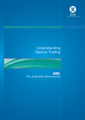
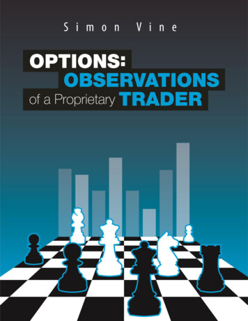
A chart of the profit and loss (P / L) profile of the portfolio (Long Put and LongUnderlying) looks like the graph of the long call position. The same is true for othersynthetic positions and their regular equivalents. It’s important to remember,however, that put/call parity works best for ATM options (50-delta).Application of synthetic positionsIf you buy 1 million of the 1.2600 EUR / USD calls (EUR call) for 150 pipswhen the EUR / USD trades at 1.2650, the call’s intrinsic value is 50 (1.2650 1.2600) pips, and its time value should be 100 pips (150 50).12As we know, the time values of calls and puts with the same strike and expiryshould be equal. Thus, if the put's price is greater than 100 pips, there is an arbitrageopportunity—i.e., you can sell the put and buy its synthetic equivalent at a gainwithout market risk for the combined position. In other words, you can sell 1million of the 1.2600 put for, let's say, 110 pips, then do a dual trade: sell 1 millionagainst the USD, and simultaneously buy the 1.2600 call at 100 pips. You will net 10(110 100) pips.Option Pricing ComponentsAlthough put / call parity helps to explain the price relationship of puts andcalls, how did investors price either before modern formulae were invented? Let’sreview a method used in the 19th century to calculate an approximate price foroptions. Back then, traders would review a few years of a stock’s previous prices andcalculate its volatility (in those days they called volatility "fluctuation"). They thenwould compare historical price fluctuations for a period equal to the option they wereconsidering. For example, they would measure a stock’s historical two-monthfluctuations if they wanted to price a two-month option. An especially scholarlytrader might also have calculated the volatility for a group of stocks within the sameindustry. She would also consider costs such as commissions, cost of capital, andperhaps a credit risk charge based on the historical default rate of counterparties.Although the aforementioned authors didn’t show calculations for OTMoptions (in those days they were called Call-of-More, while OTM puts were calledPut-of-more), we can follow their general logic to price one as they might have.Suppose the trader wants to sell a one-month call with a strike price of 120 on a stockselling at 100 (Table 1.1). Based on historical fluctuations and his forecast, hewould evaluate the probability that the stock would close within a particular price16

range within a one-month period. He would then calculate a price for the call bysumming the range of possibilities and weighting the likelihood each would occur.Table 1.1Approximate Calculation of the Option Premium (Current stock price is 100)The estimatedThe 120 call’sStock Price Range range probability inintrinsic value at1 monththe mid-range priceBelow 6060–7070–80 and 65.09.14.25.140000000Calculation of the120 call’s premium0000000Thus, assuming equal chances the stock will move up or down, the traderwould assess the option’s approximate premium at 3.875.How would the trader estimate a premium for a longer-dated option? Bywidening the underlying price ranges and the probabilities to accommodate the longerperiod. For instance, for an option expiring in two months he would consider thewider range of outcomes and different probabilities. The 120 strike would end upcloser to the middle of the distribution and thus likely would be more expensive. Forexample, the probability the stock’s price will fall within the 120– 130 rangeincreases from 0.09 to 0.12. Hence, his estimated price for the longer-term call willincrease. As we’ve noted, this 19th century calculation proved to be reasonablyaccurate when judged against today’s more complex pricing techniques.In the 1970s, the logic of the valuations above served as the basis of the CoxRubinstein Equation (1979) that values American-style options. However, the first“modern” formula for pricing European options was developed in the early 1970s byFischer Black and Myron Scholes. Their formula uses different inputs to calculatethe option’s price. They are:17

xThe price of the underlying assetxThe strike price of the optionxThe option’s expiration datexThe financing rate for the underlying stock, its rate of return (dividends inthe case of shares, coupon in the case of Eurobonds, the rate of financing ofa second currency in the case of currencies)xThe implied volatility.The next chapter goes over the principles of option pricing using theseparameters.18

CHAPTER 2COMPONENTS OF OPTIONS PRICING AND CALCULATION SHORTCUTSChapter 1 discussed basic components of options prices. They included current priceof the underlying asset, the option’s strike price, and its time to e

1720, embedded options were a part of the South Sea Company's financing schemes. In 1857, French writer Proudhon published several manuals outlining derivative trading techniques and their regulatory framework. He named call options an achete à prime and put options a vente à prime. By the 1870s, options trading had