Transcription
Synthetic Data Generation for Statistical TestingGhanem Soltana, Mehrdad Sabetzadeh, and Lionel C. BriandSnT Centre for Security, Reliability and Trust, University of Luxembourg, LuxembourgEmail: {ghanem.soltana, mehrdad.sabetzadeh, lionel.briand}@uni.luAbstract—Usage-based statistical testing employs knowledgeabout the actual or anticipated usage profile of the system undertest for estimating system reliability. For many systems, usagebased statistical testing involves generating synthetic test data.Such data must possess the same statistical characteristics asthe actual data that the system will process during operation.Synthetic test data must further satisfy any logical validity constraints that the actual data is subject to. Targeting data-intensivesystems, we propose an approach for generating synthetic testdata that is both statistically representative and logically valid.The approach works by first generating a data sample that meetsthe desired statistical characteristics, without taking into accountthe logical constraints. Subsequently, the approach tweaks thegenerated sample to fix any logical constraint violations. Thetweaking process is iterative and continuously guided towardachieving the desired statistical characteristics. We report ona realistic evaluation of the approach, where we generate asynthetic population of citizens’ records for testing a publicadministration IT system. Results suggest that our approach isscalable and capable of simultaneously fulfilling the statisticalrepresentativeness and logical validity requirements.Index Terms—Test Data Generation, Usage-based StatisticalTesting, Model-Driven Engineering, UML, OCL.I. I NTRODUCTIONUsage-based statistical testing, or statistical testing for short,is concerned with detecting faults that cause the most frequentfailures (thus affecting reliability the most), and with estimating reliability via statistical models [1]. In contrast to testingtechniques that focus on system verification (fault detection),e.g., testing driven by code coverage, statistical testing focuseson system validation from the perspective of users. Statisticaltesting typically requires a usage profile of the system undertest. This profile characterizes, often through a probabilisticformalism, the population of the system’s usage scenarios [2].Existing work on usage profiles has focused on state- andevent-based systems, with the majority of the work beingbased on Markov chains [3], [4], [5], [6], [7], [8]. For manysystems, which we refer to as data-centric and concentrate onin this paper, system behaviors are driven primarily by data,rather than being triggered by stimuli. For example, consider apublic administration system that calculates social benefits forcitizens. How such a system behaves is determined mainly bycomplex and interdependent data such as citizens’ employmentand household makeup. The system’s scenarios of use are thusintimately related to the data that is processed by the system.Consequently, the usage profile of such a system is governedby the statistical characteristics of the system’s input data,or stated otherwise, by the system’s data profile. Given ourfocus on data-centric systems and the explanation above, we978-1-5386-2684-9/17 c 2017 IEEEequate, for the purposes of this paper, “usage profile” and “dataprofile”, and use the latter term hereafter.When actual data, e.g., real citizens’ records in the aforementioned example, is available, one may be able to performstatistical testing without a data profile. In most cases, however, gaps exist in actual data, since new and retrofit systemsmay require data beyond what has been recorded in the past.These gaps need to be filled with synthetic data. To generatesynthetic data that is representative and thus suitable for statistical testing, a profile of the missing data will be required.Further, and perhaps more importantly, synthetic data (andhence a data profile) are indispensable when access to actualdata is restricted. Notably, under most privacy regulations, e.g.,EU’s General Data Protection Regulation [9], “repurposing”of personal data is prohibited without explicit consent. Thiscomplicates sharing of any actual personal data with thirdparties who are responsible for software development and testing. Anonymization offers a partial solution to this problem;however, doing so often comes at the cost of reduced dataquality [10] and proneness to deanonymization attacks [11].Data profiles have received little attention in the literature onsoftware testing. This is despite the fact that many data-centricsystems, e.g., public administration and financial systems, aresubject to reliability requirements and thus statistical testing.Recently, we proposed a statistical data profile and a heuristicalgorithm for generating representative synthetic data [12].Although motivated by microeconomic simulation [13] ratherthan software testing, our previous approach provides a usefulbasis for generating data that can be used for statistical testing.However, the approach suffers from an important limitation:while the approach generates synthetic data that is alignedwith a desired set of statistical distributions and has shownto be good enough for running financial simulations [14],the approach cannot guarantee the satisfaction of logicalconstraints that need to be enforced over the generated data.To illustrate, we note three among several other logicalanomalies that we observed when using our previous approach[12] for generating test cases based on a data profile ofcitizens’ records: children who were older than their parents, individuals who were married before being born, andindividuals who were classified as widower without everhaving been married. Without the ability to enforce logicalconstraints to avoid such anomalies, the generated data isunsuitable for statistical testing and estimating reliability. Thisis because such anomalies may result in exceptions or systembehaviors that are not meaningful. In either case, targetedsystem behaviors will not be exercised.872ASE 2017, Urbana-Champaign, IL, USATechnical ResearchAccepted for publication by IEEE. c 2017 IEEE. Personal use of this material is permitted. Permission from IEEE must be obtained for all other uses, in any current or future media, including reprinting/republishing this material for advertising or promotional purposes, creating new collective works, for resale or redistribution to servers or lists, or reuse of any copyrighted component of this work in other works.
II. BACKGROUNDIn this section, we briefly describe our previous data generation approach [12]. We leverage this approach for (1) expressing the desired statistical characteristics of data, and (2) generating initial data samples which we process further to achievenot only representativeness but logical validity as well.For specifying statistical characteristics, we use a set ofannotations (stereotypes) which can be attached to a dataschema expressed as a UML Class Diagram. Fig. 1 illustratessome of these annotations on a small excerpt of a data schemafor a tax administration system.The «probabilistic type» stereotypes applied to the specializations of the TaxPayer class state that 78% of the taxpayersshould be resident and the remainder should be non-resident.The «from histogram» stereotype attached to the birth yearattribute provides, via a histogram, the birth year distributionfor taxpayers. The attribute birth year is further annotatedwith a conditional probability specified via the «value dependency» stereotype. The details of this conditional probabilityare provided by the legal age for pensioners box. The information in the box reads as follows: 25% of pensioners havetheir birth year between 1957 and 1960, i.e., are between 57and 60 years old; the remaining 75% are older than 60.The «multiplicity» stereotype attached to the associationbetween TaxPayer and Income classes describes, via the income cardinality histogram, the distribution of the number«probabilistic type»{frequency: 0.7845}ResidentTaxPayer«probabilistic type»{frequency: 0.2155}NonResidentTaxPayerTaxPayer (abstract)- birth year : Integer«from histogram»{labels: [[1979.1998], [1959.1978], [1934.1958],[1900.1933]]; frequencies: [0.7, 0.2, 0.07, 0.03]}«value dependency»{queries: [dependency age for pensioners]}dependency age for pensioners«OCL query»{expressions: [legal age for pensioners]}income cardinality«from histogram»{labels: [1, 2, 3, 4]; frequencies:[0.8, 0.15, 0.045, 0.005]}«multiplicity»{constraints: [incomecardinality]}1 taxpayerIncomeincomes 1.*legal age for pensionersCondition: self.incomes- exists(oclIsTypeOf(Pension))«from histogram»{labels: [[1957.1960], [1917.1956]];frequencies: [0.25, 0.75]}Fig. 1. Data Schema (Excerpt) Annotated with Statistical Characteristicsof incomes per taxpayer. As shown in Fig. 1, 80% of thetaxpayers have one income, 15% have two, and so on.For generating a data sample, we previously proposed aheuristic technique that is aimed exclusively at representativeness [12]. This technique traverses the elements of thedata schema and instantiates them according to the prescribedprobabilities. The technique attempts to satisfy multiplicityconstraints but satisfaction is not guaranteed. More complexlogical constraints are not supported.In this paper, we use as a starting point the data generatedby our previous approach, and alter this data to make it validwithout compromising representativeness. Indeed, as we showin Section V, our new approach not only results in logicallyvalid data but also outperforms our previous approach in termsof representativeness.III. A PPROACH OVERVIEWFig. 2 presents an overview of our approach for generatingrepresentative and valid test data. Steps 1–3 are manual andStep 4 is automatic. In Step 1, Define data schema, we defineusing a UML Class Diagram (CD) [17] the schema of the datato generate. This diagram, illustrated earlier in Fig. 1, is thebasis for: (a) capturing the desired statistical characteristics ofdata (Step 2), and (b) generating synthetic data (Step 4).1. Definedata schemaData schema(class diagram)2. Definestatisticalcharacteristics3. Definedata validityconstraints s m The question that we investigate in this paper is as follows:Can we generate synthetic test data that is both statisticallyrepresentative and logically valid? The key challenge weneed to address when tackling this question is scalability.Specifically, to obtain statistical representativeness, we needto construct a large data sample (test suite), potentially withhundreds or thousands of members. At the same time, thislarge sample has to satisfy logical constraints, meaning that weneed to apply computationally-expensive constraint solving.Contributions. The contributions of this paper are as follows:1) We develop a model-based test data generator that cansimultaneously satisfy statistical representativeness and logical validity requirements over complex, interdependent data.The desired statistical characteristics are expressed usingour previously-developed probabilistic UML annotations [12].Validity constraints are expressed using UML’s constraintlanguage, OCL [15]. Our data generator incorporates twocollaborating components: (a) a search-based OCL constraintsolver which enhances previous work by Ali et al. [16], and(b) a mechanism that guides the solver toward satisfying thestatistical characteristics that the generated data (test suite)must exhibit.2) We evaluate our data generator through a realistic casestudy, where synthetic data is required for statistical testingof a public administration IT system in Luxembourg. Ourresults suggest that our data generator can create, in practicaltime, test data that is sound, i.e., satisfies the necessary validityconstraints, and at the same time, is closely aligned with thedesired statistical characteristics. p pAnnotateddata schemaDataprofile 4. Generatesynthetic dataOCLConstraintsSyntheticdata sample(test suite)Fig. 2. Approach for Generating Valid and Representative Synthetic DataIn Step 2, Define statistical characteristics, the CD fromStep 1 is enriched with probabilistic annotations (see Section II) to express the representativeness requirements thatshould be met during data generation in Step 4. In Step 3,Define data validity constraints, users express via the ObjectConstraint Language (OCL) [15] the logical constraints thatthe generated data must satisfy. For example, the followingOCL constraint states that children must be born at least16 years after their parents: self.children- forAll(c c.birth year self.birth year 16). Here, self refers to a person.Steps 2 and 3 of our approach can in principle be done inparallel. Nevertheless, it is advantageous to perform Step 3873
after Step 2. This is because the probabilistic annotationsof Step 2 may convey some implicit logical constraints. Forexample, the annotations of Step 2 may specify a uniform distribution over the month of birth for physical persons. It wouldtherefore be redundant to define the following OCL constraint:self.birth month 1 and self.birth month 12. Such redundanciescan be avoided by doing Steps 2 and 3 sequentially.Step 4, Generate synthetic data, generates a data sample(test suite) based on a data profile. In our approach, a dataprofile is materialized by the combination of the probabilisticannotations from Step 2 and the OCL constraints for Step 3.As stated earlier, the synthetic data generated in Step 4 mustmeet both the statistical representativeness and logical validityrequirements, respectively specified in Steps 2 and 3. Theoutput from Step 4 is a collection of instance models, i.e.,instantiations of the underlying data schema. Each instancemodel characterizes one test case for statistical testing.In the next section, we elaborate Step 4, which is the maintechnical contribution of this paper.IV. G ENERATING S YNTHETIC DATAIn this section, we describe our synthetic data generator.Fig. 3 shows the strategy employed by the data generator.Initially, a potentially invalid collection of instance models iscreated using our previous data generation approach (see Section II). We refer to this initial collection as the seed sample.Our data generator then transforms the seed sample into acollection of valid instance models. This is achieved using acustomized OCL constraint solver, presented in Section IV-A.The solver attempts to repair the invalid instance models inthe seed sample. To do so, the solver considers the constraintspecified in Step 3 of our overall approach (Fig. 2) alongsidethe multiplicity constraints of the underlying data schema andthe constraints implied by the probabilistic annotations fromStep 2 of the approach. The rationale for feeding the solverwith instance models from the seed sample, rather than havingthe solver build instance models from scratch, is based on thefollowing intuitions: (1) By starting from the seed sample, thesolver is more likely to be able to reach valid instance models,and (2) The valid sample built by the solver will not end uptoo far away from being representative, in turn making it easierto fix deviations from representativeness, as we discuss later.The OCL solver that we use is based on metaheuristicsearch. If the solver cannot fix a given instance model within apredefined maximum number of iterations, the instance modelis discarded. To compensate, the seed sample is extended witha new instance model byre-invoking our previous data generator. This process continues until we obtain the desired numberof valid instance models (test cases). The number of instancemodels to generate is an input parameter that is set by users.Once we have a valid data sample that has the requestednumber of instance models in it, our data generator attemptsto realign the sample back with the desired statistical characteristics. This is done through an iterative process, delineatedin Fig. 3 with a dashed boundary. We elaborate the details ofthis iterative process in Section IV-B.Create seedsampleSeed samplewith potentiallogical anomaliesCreate validsampleValid datasampleAll validity constraints(user-defined constraints includingOCL multiplicity constraints from dataschema plus constraints implied byprobabilistic annotations)(for each instance model in the sample)Corrective constraintsProposeGeneratetweakedcorrective Tweaked instance modelinstance modelconstraintsFinal datasampleFig. 3. Overview of our Data Generation StrategyBriefly, the process goes in a sequential manner through theinstance models within the valid sample, and subjects theseinstance models to additional constraints that are generatedon-the-fly. These additional constraints, which we refer toas corrective constraints, provide cues to the solver as tohow it should tweak an instance model so that the statisticalrepresentativeness of the whole data sample is improved.For example, let us assume that instance models representhouseholds in a tax administration system. Now, supposethat the proportion of households with no children is overrepresented in the sample. If, under such circumstances, theiterative process is working on a household with no children, acorrective constraint will be generated stating that the numberof children should be non-zero (in that particular household).The solver will then attempt to satisfy this constraint withoutviolating any of the validity constraints discussed earlier.If the solver fails to come up with a tweaked householdthat satisfies both the corrective constraint and all the validityconstraints at the same time, the original household (which isvalid but has no children) is retained in the sample. Otherwise,that is, when a tweaked and valid household is found, we needto decide whether it is advantageous to replace the originalhousehold by the tweaked one. Let I be the original householdand I 0 the tweaked one. Further, let S denote the currentsample containing I (but not I 0 ) and let S 0 (S \ {I}) {I 0 }.The decision is made as follows: If S is better aligned than S 0with the desired statistical characteristics then I 0 is discarded;otherwise, I 0 will replace I in the sample. The reason why thisdecision is required is because tweaking may have side effects.Therefore, I 0 may not necessarily improve overall representativeness, although it does reduce the proportion of householdswith no children. For example, it could be that the solver addssome children to the household in question, but in doing so, italso changes the household allowances. These allowances toomay be subject to representativeness requirements. Withoutthe comparison above, one cannot tell whether the tweakedhousehold is a better fit for representativeness.In the above scenario, we illustrated the iterative processusing a single corrective constraint. In practice, the processmay generate multiple such constraints, since the data sampleat hand may be deviating from multiple representativenessrequirements. We treat corrective constraints as being soft.This means that if after the maximum number of iterations,the solver manages to solve some of the corrective constraintsbut not all, the process will give the tweaked instance model874
a chance to replace the original one as long as the tweakedinstance model still satisfies all the validity constraints.The rest of this section presents the technical machinerybehind the (customized) OCL solver and our data generator.A. Solving OCL ConstraintsA number of techniques exist for solving OCL constraints,notably using Alloy [18], [19], constraint programming [20],and (metaheuristic) search [21], [16]. Alloy often fails tosolve constraints that involve large numbers [22]. We observedvia experience that this limitation could be detrimental inour context. For example, our case study in Section V hasseveral constrained quantities, e.g., incomes and allowances,that are large numbers. As for constraint programming, to ourknowledge, the only publicly-available tool is UML2CSP [20].We observed that this tool did not scale for our purposes. Inparticular, given a time budget of 2 hours, UML2CSP did notproduce any valid instance model in our case study. This is notpractical for statistical testing where we need a representativesample with many (hundreds or more) valid instance models.Search, as we demonstrate in Section V, is more promisingin our context. Although search-based techniques cannot prove(un)satisfiability, they are efficient at exploring large searchspaces. In our work, we adopt with two customizations thesearch-based OCL solver of Ali et al.’s [16], hereafter referredto as the baseline solver. The customizations are: (1) a featurefor setting a specific instance model as the starting point forsearch, and (2) a strategy to avoid premature narrowing of thesearch space. The former customization, which is straightforward and not discussed here, is necessary for realizing theprocess in Fig. 3. The latter customization is discussed next.The baseline solver has a fixed heuristic for selecting whatOCL clause to solve next: it favors clauses that are closerto being satisfied based on a fitness function. For example,assume that we want to satisfy constraint C1 defined asfollows: if (x 2) then y 5 else if (x 3) then y 4 else y 0 endif endif,where x and y are attributes. For the sake of argument, supposethe solver is processing a candidate solution where x 3(satisfying the condition of the second nested if statement)and y 7 (not satisfying any clause). This makes the secondnested if statement in C1 the closest to being satisfied. At thispoint, the heuristic employed by the solver narrows the searchspace by locking the value of x and starting to exclusivelytweak y in order to satisfy y 4. Now, if we happen to haveanother constraint C2 stating y 4, the solver will fail since xcan no longer be tweaked.The above heuristic in the baseline solver poses no problemas long as the goal is to find some valid solution. If search failsfrom one starting point, the solver (pseudo-)randomly picksanother and starts over. In our context however, starting overfrom an arbitrary point is not an option. For the final datasample to have a chance of being aligned with the desiredstatistical characteristics, the solver needs to use as startingpoint instance models from a statistically representative seedsample (see Fig. 2). If the solver fails at making valid aninstance model from the seed sample, that instance model hasto be discarded. This negatively affects performance, since thesolver will need to start all over on a replacement instancemodel supplied by the seed data generator, as noted earlier.In a similar vein, if the solver fails at enforcing correctiveconstraints over a (valid) instance model, it cannot helpwith improving representativeness. To illustrate, suppose thatconstraint C2 mentioned earlier is a corrective constraint andthat the valid solution (instance model for C1) is x 3, y 4.In such a case, the baseline solver will deterministically failas long as the starting point is this particular valid solution.In other words, C2 will have no effect.To address the above problem, we customize the baselinesolver as follows: Rather than working directly on the originalconstraints, the customized solver works on the constraints’prime implicants (PI). An implicant is prime (minimal) ifviolating any of its literals results in the violation of theunderlying constraint. To derive all the PIs for a given OCLconstraint, we first transform the constraint into a logicalexpression with only ANDs and ORs, negation, and OCLoperations. We next transform this expression into DisjunctiveNormal Form (DNF) by applying De Morgan’s law [23]. Eachclause of the DNF expression is a PI. For instance, constraintC1 yields three PIs: (x 2 and y 5), (x 2 and x 3 and y 4), and(x 2 and x 3 and y 0). Note that we use the term PI slightlydifferently than what is standard in logic. Our literals are notnecessarily independent logically. For example, in the secondPI above, x 2 is redundant because x 3 implies x 2. Suchredundancies pose no problem and are ignored.For each constraint C to be solved, the customized solverrandomly picks one of C’s PIs. For instance, if we want tosolve constraints C1 and C2 together, we would randomly pickone of C1’s three PIs alongside C2 (whose only PI is y 4). Thisway, we give a chance to all PIs to be considered, thus avoidingthe undesirable situation discussed earlier, where the baselinesolver would (deterministically) lead itself into dead-ends. Forexample, from the PIs of C1, we may pick (x 2 and y 5). Now,if we start the search at x 3, y 7, the solver will havea feasible path toward a valid solution, x 2, y 5, whichsatisfies both C1 and C2. If a certain combination of randomlyselected PIs (one PI per constraint) fails, other combinationsare tried until either a solution is found or the maximumnumber of iterations allowed is reached.Due to space, we cannot present all the details of thiscustomization. We only make two remarks. First, all OCLoperations are treated as opaque literals when building PIs.For example, the operation self.navigation forAll(x 3 or y 2) isa single literal, just like, say, x 3. Solving OCL operationsis a recursive process and similar to solving operation-freeexpressions. In particular, to solve OCL operations, we employthe same DNF transformation discussed earlier. For example,to solve self.navigation forAll(x 3 or y 2), we derive two PIs,x 3 and y 2, and use them to constrain the objects at theassociation end that has navigation as role name.Second, the DNF transformation can result in exponentiallylarge DNF representations when there are many literals [24].Such exponential explosion is unlikely to arise in our context:875
Manually-written logical constraints for data models typicallyinclude only a handful of literals. For the corrective constraintsthat are generated automatically (through Alg. 2 describedlater), the number of literals is at most as many as thenumber of ranges (or categories) in the bar graphs that capturethe desired statistical distributions. Again, these numbers areseldom very large. In our case study of Section V, the DNFtransformations took negligible time (milliseconds).To summarize, using PIs instead of the original constraintshelps avoid dead-ends when solution search has to start froma specific point in the search space. In Section V (RQ1), weexamine how customizing the baseline solver in the mannerdescribed in this section influences performance.Alg. 1: Process Instance Model (PIM): (1) a set S of valid instance models; (2) an instance modelinst S to process; (3) a set V of validity constraints;(4) a set Hdesired of desired statistical characteristics(expressed as histograms); (5) a parameter nb attemptsdenoting the number of times that the solver will beinvoked over inst to create tweaked instance models; (6) aparameter freq sensitivity [0.1] denoting the marginbeyond which two relative frequencies are deemed far apart./* freq sensitivity is used only for invoking GCC (Alg. 2). */Output: Either inst or a tweaked instance model, whichever leads toa more representative data sample.Fun. calls: GCC: generates corrective constraints (Alg. 2);solve: invokes the customized solver (see Section IV-A).12B. Generating Valid and Representative Data3This section presents the technical details of our datageneration strategy, depicted in Fig. 3 and outlined earlier on.We already discussed the creation of the seed sample (from ourprevious work [12]) and how we make this sample valid usinga customized OCL solver (Section IV-A). Below, we focus onthe iterative process in Fig. 3, i.e., the region delineated bydashed lines, and present the algorithms behind this process.We start with some remarks about how we representstatistical distributions. The instruments we use to this endare barcharts (for categorical quantities) and histograms (forordinal and interval quantities). Without loss of generality,and while we support both notions, we talk exclusively abouthistograms in the text. A histogram is a set of bins. Each binis defined by a label (value or range), and a relative frequencydenoting the proportional abundance of the bin’s label. We donot directly handle continuous distributions, e.g., the normaldistribution. Continuous distributions are discretized into histograms. Doing so is routine [25] and not explained here. Wenote however that the discretization should not be too finegrained, e.g., resulting in more than 100 bins. This is becausethe corrective constraints in our approach will get complex,in turn posing scalability issues for the OCL solver, e.g., withrespect to the DNF transformation discussed in Section IV-A.The PIM algorithm. Alg. 1, Process Instance Model (PIM),presents the procedure for one iteration of the iterative process(region within the dashed boundary) in Fig. 3. PIM takes thefollowing as input: (1) a valid data sample, (2) a specificinstance model from the sample to process, (3) a set of validityconstraints, (4) the desired statistical characteristics defined ashistograms, (5) a parameter specifying how many attempts thealgorithm should make to generate tweaked instance models,and (6) a parameter specifying how sensitive the algorithm isto differences in relative frequencies. Essentially, if the difference between two relative frequencies is below the sensitivityparameter, the two frequencies are considered equal.The algorithm works in three stages as we describe next.1) Generate corrective constraints (L. 1-3 of Alg. 1): In thisstage, PIM calls another algorithm GCC (Alg. 2, describedlater). GCC generates corrective constraints for the instancemodel being processed (L. 1). For example, assume thatthe instance model is a pensioner, and that pensioners areInputs456789101112131415161718CC GCC(S, inst, Hdesired , freq sensitivity)/* CC is the set of corrective cons
The desired statistical characteristics are expressed using our previously-developed probabilistic UML annotations [12]. Validity constraints are expressed using UML's constraint language, OCL [15]. Our data generator incorporates two collaborating components: (a) a search-based OCL constraint solver which enhances previous work by Ali et al .