Transcription
Wavelet-Based Poisson Solver for Use in Particle-in-Cell SimulationsBalša Terzić Department of Physics, Northern Illinois University, DeKalb, Illinois 60115Ilya V. PogorelovAccelerator and Fusion Research Division, Lawrence Berkeley National Laboratory(Dated: May 11, 2005)We report on a successful implementation of a wavelet-based Poisson solver for use in 3D particlein-cell simulations. Our method harnesses advantages afforded by the wavelet formulation, such assparsity of operators and data sets, existence of effective preconditioners, and the ability simultaneously to remove numerical noise and further compress relevant data sets. We present and discusspreliminary results of application of the new solver to test problems in accelerator physics andastrophysics.KEYWORDS: multiscale dynamics, wavelets, N-body simulations, particle-in-cell method, Poisson equationI.tion is several orders of magnitude smaller than thenumber of particles in the physical system which isbeing modeled; andINTRODUCTIONGaining insight into the dynamics of multiparticle systems, such as charged particle beams or self-gravitatingsystems, heavily relies on N-body simulations. Themany-body codes can be grouped into three main categories: (i) direct summation, (ii) tree and (iii) particlein-cell (PIC). The direct summation codes are prohibitively expensive for large systems, since their computational cost scales as N 2 . The tree codes use directsummation for nearby particles and evoke statistical arguments for contribution of particles farther away. ThePIC codes incorporate a computational grid into whichparticles are binned, thus resulting in the coarse-grained,discretized particle distribution. The potential associated with such discretized particle distribution is computed by solving the Poisson equation on the grid. Finally, the forces needed to advance each individual particle are computed by interpolation from the discretizedpotential on the grid. A detailed treatment of computational methods to simulate multiparticle systems is givenby Hockney and Eastwood [1]. In this paper we outline awavelet-based algorithm for solving the Poisson equationfor use in PIC codes.It is important that the algorithms used in solving thePoisson equation:1. account for multiscale dynamics, because even thefluctuations on smallest scales can lead to globalinstabilities and fine-scale structure formation, asexemplified by halo formation and microbunchinginstability observed in beam dynamics experiments[2–5],2. minimize the numerical noise due to the fact thatthe number of particles used to sample the phasespace distribution function in the N -body simula-3. be as efficient as possible in terms of computationalspeed and storage requirement, without compromising accuracy.Furthermore, for some important applications, such ascoherent synchrotron radiation (CSR) in beam dynamics,it is necessary to have a compact representation of thesystem’s history [5, 6].The wavelet-based solver we present here has the potential to satisfy all of the requirements listed above. InSection II we briefly outline the concept of wavelets andwavelet transforms. Formulating the Poisson equationon the grid and solving it using the wavelet-based approach is reported in Section III. In Section IV, we begin by applying the wavelet-based solver to model twodensity distributions of interest in beam dynamics andastrophysics. We then proceed to replace (for testingpurposes) the Green’s function-based Poisson solver inIMPACT-T beam dynamics code [7, 8] with the waveletbased solver, and compare results produced by the twoversions of IMPACT-T evolving the same initial distributions. We conclude with a summary of the work presented and a description of the work in progress.II.WAVELETS AND WAVELET TRANSFORMSWavelets and wavelet transforms are a relatively newconcept, introduced in the 1980’s [9–12]. The discretewavelet transform can be viewed in two different ways,as: Correspondingauthor.Email addresses: bterzic@nicadd.niu.edu, ivpogorelov@lbl.gov1. the discrete analog of the continuous wavelet trans-
2and the inverse Laplacian operators are sparse;also, the iterative methods can be accelerated using preconditioners that are effectively diagonal inwavelet bases [13–15].III.WAVELET-BASED POISSON SOLVERThe Poisson equation solved by the PIC codes is defined on a computational grid which contains all the particles used in the simulation. The discretization takesthe Poisson equation with Dirichlet boundary conditions(BCs), i.e., for which the value of the function is specifiedon the boundary, from its continuous form52 u f,FIG. 1: Affect of the initial guess on the preconditioned conjugate gradient method. The rate of convergence remains thesame, given by eq. 5, while it is obvious that a better initial guess leads to convergence to the desired accuracy withinsignificantly fewer steps.form of a function f (t) given byg(s, x) Z f (t)Ps,x (t)dt,(1) 1Ps,x (t) Ps t xs ,(2)where P (t) is a mother wavelet, from which thewavelet basis functions are computed by scalingand/or translation [12].2. a family of perfect reconstruction high- and lowpass filters, which can extract information from thesignal at varying scales. Then the forward andinverse discrete wavelet transforms can be represented by filtering and down- or up-sampling, respectively [10, 11].There are three main reasons that a wavelet-basedPoisson solver is of interest:1. Solving the problem in wavelet space enables retaining information about the dynamics on different scales spanned by the wavelet expansion.2. Wavelet formulation also allows for natural removing numerical noise (denoising) through thresholding the wavelet coefficients. This also reduces theeffective dimensionality of the problem, thereby reducing the computational load.3. Formulating and solving the Poisson boundaryvalue problem in wavelet space provides considerable computational speedup: both the Laplacianubnd h(3)where 52 is the continuous Laplacian derivative, toLU F,Ubnd H(4)where the Laplacian operator L, potential U , density Fare all defined on the computational grid and H is specified on the surface of the grid. Eq. (4) represents a wellknown problem in numerical analysis. It can be solvedusing a number of iterative methods, such as multigrid,successive over-relaxation, steepest descent, or conjugategradient. For the work presented here, we generalized to3D the preconditioned conjugate gradient (PCG) method[16, 17]. The PCG method iteratively updates the initial solution along the conjugate directions until the exitrequirement LU F 2 2 F 2 ,(5)is satisfied in some norm 2 . The convergence rate of themethod is dependent on the condition number (k) of theoperator L:U Ui2 !i k 1 U 2 ,k 1(6)where U i is the approximation to the exact solution Uafter the ith iteration. The smaller the condition number, the faster the approximation U i approaches to theexact solution U . The condition number k of the Laplacian operator L on a grid is proportional to the squareof the grid resolution, k(L) O(N 2 ), where N is thenumber of cells in each coordinate. Such large conditionnumber results in a slowly-converging scheme. However,in wavelet space, there is an effective diagonal preconditioner P for the wavelet-transformed Laplacian operatorLw , which reduces the condition number of the preconditioned operator to k(P Lw P ) O(N ) [13–15]. Thisprovides a significant computational speedup.Whereas the rate of convergence is set by the relationgiven in Eq. (6), the number of iterations needed to attain a certain predefined accuracy also depends on how
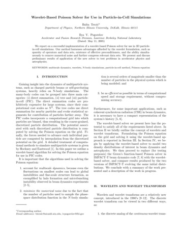
3FIG. 2: Flow-chart outline of the wavelet-based Poisson solver using the (constrained) PCG method. The gray boxes representthe wavelet-space; the physical space is in white. Constraining of the PCG method is done in the bottom middle box. Thecurrent version of the code does not have this step implemented yet.close the initial guess is to the solution. Since one doesnot expect significant changes in the potential from oneinstant in time t t0 to the next t t0 t, the potential at t t0 serves as a good initial guess for theconjugate gradient iteration at t t0 t. The importance of having a “smart” initial guess is illustrated inFigure 1.Thresholding the wavelet coefficients (setting themequal to zero if their magnitudes are below a certainpredefined threshold) can be used to remove the smallest scale fluctuations usually associated with numerical noise. It is worth remembering, however, that essential physics that must be captured in a typical PICsimulation includes various instabilities and fine structure/substructure formation. These processes owe theirexistence to the coupling between multiple spatial scaleson which the system’s dynamics unfolds. Uncontrolleddenoising carries with it the obvious danger of “smoothing out” the fine-scale details that serve as seeds for theonset of these processes. Still, there are numerous indications that properly implemented adaptive denoisingcan enable significant reduction in the size of the relevant data sets without compromising the solver’s abilityto resolve the physically important multiscale aspects ofthe system’s dynamics. Denoising-by-thresholding effectively reduces (constrains) the search space for the iterative PCG method. Our implementation of the constrained PCG (CPCG) will be reported elsewhere.A schematic representation of the solver is given inFigure 2.A.Implementing Boundary ConditionsIn the current implementation, we take the beam topass through a grounded rectangular pipe. Over the fourwalls of the pipe, U 0, and the two open ends throughwhich the beam passes have open BCs. We choose thecomputational grid to have dimensions 3-10 times smallerthan those of the pipe, and we compute the potential overthe six surfaces of this grid using a Green function whilesatisfying the constraints on U that the pipe imposes.
4FIG. 3: Plummer sphere particle distribution (top left) and corresponding potential (top right) obtained using the PCG. Thelower panels show two convergence criteria correction at the next iteration (bottom left) and how well the difference equationis satisfied (bottom right) with (solid line) and without the preconditioner (dashed line).Accordingly, the computation of BCs reduces to solvingthe following system of equations [8]:ρlm4(z) abZa Zb0ρ(x, y, z) sin(αl x) sin(βm y)dydx, (7)0 2 φlm (z)ρlm (z)2 γlmφlm (z) ,2 z 0φ(x, y, z) NxNx XXl 1 l 1φlm (z) sin(αl x) sin(βm y),(8)(9)where ρ is the charge distribution, φ is the potential, αl 22lπ/a, βm mπ/b, γlm α2l βm, 0 is the permittivityof vacuum and the geometry of the pipe is given by 0 x a and 0 y b [8]. Eq. (9) is evaluated onlyon the surface of the computational grid, and for thepredefined number of expansion coefficients Nx and Ny ,thus yielding Ubnd from Eq. (4). This is only one of theways to compute the potential on the surface of the grid.Others, more efficient and computationally cheaper, willbe a implemented in the future editions of the code.The PCG solves Eq. (5) assuming U 0 outsidethe computational grid. The inhomogeneous Dirichletboundary-value problem in Eq. (4) has been made equivalent to the homogeneous one by transferring the inhomogeneous boundary value terms to the source. In the
5FIG. 4: Particle distribution (top left) and corresponding potential (top right) for the “fuzzy cigar” obtained using the PCG.The lower panels show two convergence criteria correction at the next iteration (bottom left) and how well the differenceequation is satisfied (bottom right) with (solid line) and without the preconditioner (dashed line).simplest case where the spacing of the computational grid is the same in x-, y- and z-directions, the altered sourcebecomes F F H/ 2 [18].Plummer spherical stellar distribution (Figure 3). Boththe potential and density are analytically known and aregiven byF (r) IV.APPLICATIONSOur goal has been to develop a wavelet-based Poisson solver which can be easily merged into existing PICcodes designed for multiparticle dynamics simulations.As the first step towards that goal, we tested the solveron two idealized particle distributions, one from astrophysics and the other from beam dynamics. We used thePCG solver to compute the potential associated with the3,U (r) 1,1 r2(10)(1 pwhere r x2 y 2 z 2 . The potential on the surfaceof the computational grid is specified analytically. Thebottom panels of the Figure 3 demonstrate the substantial computational speedup gained by preconditioning.Here we applied open BCs, U (r ) 0, which is thenatural choice for self-gravitating systems.We then applied the algorithm to a more realistic setting in which only the particle distribution is analytically5r2 ) 2
6Initial particle distribution; N 200,000IMPACT-T: 0.50Y(mm-0.5 -1) -1.5-2 -2-0.5 0-1.5 -10.511.523Y ( 2.5 2mm 1.5))X (mmIMPACT-T with PCG (N x Ny 30): Potential10.50.51 1.532 2.53.5 4)X (mmIMPACT-T with PCG (N x Ny 100): 532.5Y(mm21.5)10.50.532 2.51 1.5)3Y ( 2.5 2mm 1.5)3.5 4X (mm10.50.51 1.532 2.53.5 4)X (mmFIG. 5: z-integrated non-axisymmetric particle distribution (top left) for a beam. The other panels show the correspondingpotential computed using the Green’s function method used in the standard IMPACT-T (top right), IMPACT-T with PCGand Nx Ny 30, i.e. 900 coefficients in the Green’s function expansion of the potential on the surface of the computationalgrid (bottom left) and IMPACT-T with PCG and Nx Ny 100 (bottom right).known, and where the potential on the surface of the computational grid is computed using the analytically knownGreen’s function (Figure 4). It is an axially symmetric“fuzzy cigar”-shaped configuration of charged particles(a “beam bunch”) given byF (x, y, z) d1 (R)d2 (z),d1 (R) 1(R R2 )2 (R (3R1 2R2 ))24(R1 R2 )4 0(11)0 R R1 ,R1 R R 2 , .otherwise,(12) 1z1,2 z z2,1 , (z z1 )2 (z (3z1,2 2z1 ))2 z z z ,11,24(z1,2 z2 )4d2 (z) .(z z2 )2 (z (3z2,1 2z2 ))2 z2,1 z z2 , 44(z z) 2,12 0otherwise,(13)where and the beam parameters R1 , R2 , z1 , z2 , z1,2 ,z2,1 are chosen so that 0 R1 R2 and z1 z1,2 z2,1 z2 . We applied BCs of a grounded rectangular pipein the transverse direction (i.e., U 0 on the pipe walls),and open in the longitudinal (z) direction. Similarly tothe case of the Plummer sphere, a high accuracy solutionis obtained in about 30 iterations of the algorithm witha preconditioner, or about 60 without.Upon successfully testing the PCG as a standalone Poisson solver, we replaced the standard Green’sfunction-based Poisson solver in the PIC code IMPACT-
73σx (mm) x,n (mmm-mrad)3503002.52502002IMPACT-T w/ CPCG 100IMPACT-T w/ CPCG 30IMPACT-T1.5150100IMPACT-T w/ CPCG 100IMPACT-T w/ CPCG ition (m)1.40.10.150.20.250.30.35z-position (m)σz,n (mm)24221.2 z,n (ps-keV)2018116140.8120.610IMPACT-T w/ CPCG 1000.4IMPACT-T w/ CPCG 308IMPACT-T6IMPACT-T w/ CPCG 100IMPACT-T w/ CPCG on (m)000.050.10.150.20.250.30.35z-position (m)FIG. 6: Simulation results for the radio frequency gun of the Fermilab/NICADD photoinjector done with the standard versionof IMPACT-T (solid lines), IMPACT-T with PCG with Nx Ny 30 (dashed line) and IMPACT-T with PCG with Nx Ny 100 (dotted line): rms beam radius (top left), rms normalized transverse emittance (top right), rms bunch length (bottomleft), rms normalized longitudinal emittance (bottom right). The close agreement indicates that both codes launch the beamin essentially identical fashion; this is critically important because the output of the full photoinjector depends sensitively onthe “initial conditions”.T [7, 8] with the PCG. For algorithm testing purposes,our solver uses Green’s functions to evaluate the potentialonly on the surface of the computational grid, and thenproceeds with the PCG algorithm to compute the potential on the interior. This introduces a certain computational inefficiency that will be eliminated, at the stageof optimizing the solver for performance, by using a different approach for computing BCs. The details of thisoptimization will be reported elsewhere. The parameters Nx and Ny specify the number of Green’s functionexpansion coefficients in x- and y-directions. The BCs,again, correspond to a grounded rectangular pipe in thetransverse directions, and open in the longitudinal direction. In a typical simulation, the cross-section of the pipeis larger than the cross-section of the computational gridby a factor of 3-10.In Figure 5, we compare the Green’s functions-basedPoisson solver used by IMPACT-T with the PCG byplotting the potential each algorithm computes from thesame initial particle distribution. For the simulationsdone with the wavelet-based Poisson solver, no waveletcoefficient thresholding was done, i.e., the full waveletexpansion is retained. The thresholding and the resulting denoising will be developed and implemented in thefinal version of the code.We tested our wavelet-based code in the context of theFermilab/NICADD photoinjector using 200,000 simulation particles and a nonuniform initial particle distribution at the cathode. It appears that not specifying thepotential on the surface of the grid accurately enough
814σx (mm)3IMPACT-T w/ CPCG2.5 x,n (mm-mrad)1210IMPACT-T281.56140.52IMPACT-T w/ CPCG002468IMPACT-T00123z-position (m)1.8σz,n (mm)901.656789 z,n (ps-keV)801.4701.2601500.8IMPACT-T w/ CPCG0.640IMPACT-T w/ CPCG30IMPACT-TIMPACT-T0.4200.204z-position (m)100246z-position (mm)800246z-position (mm)8FIG. 7: Simulation results for the full Fermilab/NICADD photoinjector done with the standard version of IMPACT-T (solidlines) and IMPACT-T with PCG with Nx Ny 30 (dashed line): rms beam radius (top left), rms normalized transverseemittance (top right), rms bunch length (bottom left), rms normalized longitudinal emittance (bottom right).causes considerable smoothing of the smaller scale features as computed by the wavelet algorithm. This, however, does not significantly affect the root mean square(rms) properties of the beam (Figures 6 and 7), as confirmed by the excellent agreement between simulationruns done with standard IMPACT-T (solid line) andIMPACT-T with a wavelet-based Poisson solver withNx Ny 30, i.e., 900 expansion coefficients (dashedline). The difference between the simulations with thestandard IMPACT-T (solid line) and IMPACT-T witha wavelet-based Poisson solver with Nx Ny 100 isalmost imperceptible (Figure 6).These results clearly demonstrate that the simulations using wavelet-based Poisson solver and the standard IMPACT-T are in excellent agreement in regard tothe compuation of beam moments. This establishes thepresent study as an important proof-of-concept.V.DISCUSSION AND CONCLUSIONWe formulated and implemented a prototype, 3D,wavelet-based Poisson solver that uses the preconditionedconjugate gradient method. The idea of combining thewavelet formulation and PCG to solve the Poisson equation is not new: there have been pioneering implementations of wavelet-based solvers for the Poisson equationwith homogeneous (U 0) Dirichlet BCs in 1D [13] andperiodic BCs in 1D, 2D and 3D [14, 15]. We built onthis earlier work to design and implement a solver for thethree-dimensional Poisson equation with general inhomogeneous Dirichlet boundary conditions. This constitutesan original contribution on our part, since the formulation of the discretized problem, which includes the treatment of the boundary conditions and the Laplacian operator, differs significantly from the periodized problem.Having first tested our method as a stand-alone solver
9on two model problems, we then merged it into IMPACTT to obtain a fully functional serial PIC code. We foundthat simulations performed using IMPACT-T with the“native” Poisson solver (based on Green’s functions andfast Fourier transforms) and IMPACT-T with the PCGsolver described in this paper produce essentially equivalent outcomes (in terms of a standard set of rms diagnostics). This result enables us to move from theproof-of-concept stage to the advanced optimization andapplication-specific algorithm design. To our knowledge,the work reported here constitutes the first applicationof the wavelet-based multiscale methodology to 3D computer simulations in beam dynamics.Our current efforts are focused on several areas thatencompass both algorithm optimization and applicationswork. On the optimization side, the top priority is toenable efficient computation of the potential over theboundary of the computational grid (as distinct fromthe physical boundaries of the system). Another priority is incorporation into the solver of state-of-the-artroutines for efficient storage and multiplication of multidimensional sparse arrays. Next, adaptive denoising (andsimultaneous compression) in the context of PIC modeling presents us with a unique set of technical challengesand a wealth of complex and engaging multiscale physics.Finally, we have not yet addressed the complex issues ofsolver parallelization for use with the parallel version ofIMPACT-T on multiprocessor machines.On the side of applications, we are working on leveraging the advantages afforded by the multiscale waveletformulation to tackle the previously all but intractable– in the sense of being prohibitively expensive computationally – problem of high-precision 3D modeling of CSRand its effects on the dynamics of beams in a varietyof accelerator systems. The details of our approach willbe reported, together with the first results, in the nearfuture.[1] R. Hockney and J. Eastwood, Computer Simulations Using Particles (Institute of Physics Publishing, London,1988).[2] C. A. et al., Phys. Rev. Lett. 89, 214802 (2003).[3] C. Bohn and I. Sideris, Phys. Rev. Lett. 91, 264801(2003).[4] J. Qiang, R. Ryne, and I. Hofmann, Phys. Rev. Lett. 92,174801 (2004).[5] Z. Huang, M. Borland, P. Emma, J. Wu, C. Limborg,G. Stupakov, and J. Welch, Phys. Rev. ST Accel. Beams7, 074401 (2004).[6] C. Bohn, AIP Conference Proceedings 647, 81 (2002).[7] J. Qiang, R. Ryne, S. Habib, and V. Decyk, J. Comp.Phys. 163, 434 (2000).[8] J. Qiang and R. Ryne, Comp. Phys. Comm. 138, 18(2001).[9] S. Goedecker, Wavelets and Their Applications (Pressespolytechniques et universitaires romandes, Lausanne,1998).[10] M. Misiti, Y. Misiti, G. Oppenheim, and J. Poggi,Wavelet Toolbox for Use with MATLAB (The MathWorks, Inc., Natick, Massachusetts, 1997).[11] M. Wickerhauser, Adaptive Wavelet Analysis From The-ory to Software (A K Peters, Wellesley, Massachusetts,1994).I. Daubechies, Ten Lectures on Wavelets (SIAM,Philadelphia, 1992).G. Beylkin, In Wavelets: Mathematics and Applications,eds. J. Benedetto and M. Frazier (CRC Press LLC, BocaRaton, Florida, M.Israeli(2003),http://www.cs.tau.ac.il/ amir1/PS/poisson.pdf.A. Averbuch, G. Beylkin, R. Coifman, P. Fischer, andM. Israeli, In Signal and Image Representation in Combined Spaces, eds. Y. Zeevi and R. Coifman (AcademicPress, San Diego, 1998).G. Golub and C. V. Loan, Matrix Computations (JohnsHopkins University, Baltimore and London, 1996).M. Hestines and E. Stiefel, J. Res. Nat. Bur. Stand. 49,409. 49, 409 (1996).W. Press, S. Teukolsky, W. Vetterling, and B. Flannery, Numerical Recipes in Fortran: The Art of ScientificComputing, 2nd edition (Press Syndicate of the University of Cambridge, Cambridge, 1992).Acknowlegements. Both authors are thankful toHenry Emil Kandrup for the role he played in their lives.His thoughtful guidance and patient mentorship greatlyinfluenced their scientific careers. It is through him thatthis collaboration was established in the first place.The authors are grateful to Daniel Mihalcea for running the numerical simulations and generating the Figures 5-7. Ji Qiang provided valuable help in integratingthe solver into the IMPACT-T suite. We are thankful toCourtlandt Bohn for useful and stimulating discussionsand comments. Balša Terzić was supported by the AirForce contract FA9471-040C-0199. The work of Ilya V.Pogorelov was supported by the Director, Office of Science, of the U. S. Department of Energy under contractNo. DE-AC03-76SF00098.[12][13][14][15][16][17][18]
Poisson solver is of interest: 1. Solving the problem in wavelet space enables re-taining information about the dynamics on di er-ent scales spanned by the wavelet expansion. 2. Wavelet formulation also allows for natural remov-ing numerical noise (denoising) through threshold-ing the wavelet coe cients. This also reduces the