Transcription
Preprint of the accepted submission toInformation Sciences,to be published in 2004.Evolutionary and Alternative Algorithms:Reliable Cost Predictions for Finding Optimal Solutionsto the LABS Problem Franc Brgleza,1 , Xiao Yu Lia , Matthias F. Stallmanna , Burkhard MilitzerbabComputer Science Department, NC State University, Raleigh, NC 27695, USACarnegie Institution of Washington, Washington, DC 20015, USAAbstractThe low-autocorrelation binary sequence (LABS) problem represents a major challenge to all search algorithms, with the evolutionary algorithms claiming the best resultsso far. However, the termination criteria for these types of stochastic algorithms arenot well-defined and no reliable claims have been made about optimality. Our approachto find the optima of the LABS problem is based on combining three principles intoa single method: (1) solver performance experiments with problem sizes for which optimal solutions are known, (2) an asymptotic statistical analysis of such experiments,(3) reliable predictions of the computational cost required to find optimal solutions forlarger problem sizes. The proposed methodology provides a well-defined terminationcriterion for evolutionary and alternative search algorithms alike.keywords: fundamental combinatorial algorithms, performance predictions and evaluations, low-autocorrelation binary sequence, evolutionary algorithms Ready-to-execute software environment, data sets, and the results reported in the experimentshave been archived on the LABS problem home page www.cbl.ncsu.edu/OpenExperiments/LABS/Email , stallmann@cs.ncsu.edu,Corresponding author.1militzer@gl.ciw.edu
1IntroductionThe low-autocorrelation binary sequence (LABS) problem has a simple formulation. Consider a binary sequence of length L, S s1 s2 . . . sL and their autocorrelations Ck (S) PL ki 1 si si k , si { 1, 1}, for k 1, . . . , L 1. The energy function of interest isE(S) L 1XCk2 (S)(1)k 1which defines the merit factor F of the sequence [1]:F L2 /(2E).(2)The objective of optimization is to find a sequence that maximizes F , or equivalently,minimizes E. Finding an optimum sequence has important applications in communicationengineering and is also of interest to physicists since the sequence models one-dimensionalsystems of Ising-spins. The solution of the LABS problem corresponds to the ground stateof a generalized one-dimensional Ising spin system [2]. The problem as formulated in (1)is NP-hard or worse, unlike the special cases of the Ising spin-glass problems with limitedinteraction and periodic boundary conditions evaluated in [3, 4]. While efficient and effectivemethods have been presented to solve the special cases up to L 400 [3, 4], the optimalmerit factors for the problem as formulated in (1) are presently known for values of L 60only [5, 6]. The difficulty of the LABS problem arises not only from the inconsistency orfrustration of different energy interaction terms [7] but also from the fact that for mostvalues of L, the number of global optima is relatively small, as shown in Table 1. Theresults as reported in Table 1 are a by-product of the approach we introduce in this paper.The asymptotic value for the maximum merit factor F is known [1] and has also beenre-derived using arguments from statistical mechanics [2]: as L , F 12.3248. InFigure 1, we plot the currently known values of the merit factor as the function of L,normalized with respect to 12.3248. The values for L 60 are based on a branch-andbound solver and are thus known to be optimal [5, 6]. For L 60, the values are basedon the best known merit factors reported by stochastic search solvers [8, 9, 10, 11, 12], andalso on the work in this paper. It shoud be noted that these results are significantly betterthan the solutions based on simulated annealing in [2].Table 1: The number of optimal sequences for the LABS problem. The values listed forL 35 are exact. For L 35, the values are based on our experiments to date. Some arerounded to the nearest integer multiple of 4. For odd values of L, the number of optimalsequences that are skew-symmetric is shown between the 2(4)12(4)
1.2(merit factor)/12.324810.80.6optima0.4other heuristicour heuristic0.20asymptotic value410100L, the low autocorrelation binary sequence (LABS) length1000Figure 1: Exact optima and the best known figures of merit for the low autocorrelation binarysequences, normalized to the asympotic limit of 12.3248. The exact optima are known only forL 60. The regression line is based on the least-square fit to the data points shown. Thereclearly is a significant ‘gap of opportunity’ for the new generation of LABS solvers, startingat L 100.The simple formulation and the known asymptotic value for large values of L makes theLABS problem a particularly interesting case of a problem that is most likely NP-hard orworse. As depicted in Figure 1, the problem presents a significant challenge not only tothe branch-and-bound solvers but also to the stochastic solvers: while the exact figures ofmerit, limited to values of L 60, follow the expected trend, the figures of merit reportedby current heuristics for values of L 100 are clearly diverging from the expected trend.Questions that arise include: (1) are the current stochastic solvers inadequate for the task,(2) are the solvers being terminated prematurely, and (3) is the current trend due to somecombination of (1) and (2). We argue that the most likely answer is (3) and that theproblems for L 100 may be solved better with improved solver technology. Consider, forexample, the advances in solving problems in satisfiability (SAT). Real-world SAT problemswith 100s of decision variables can today be solved routinely and reliably using branch-andbound SAT solvers as well as stochastic SAT solvers [13].Our approach to finding the optima of the LABS problem is based on combining threeprinciples into a single method: (1) solver performance experiments with problem sizes forwhich optimal solutions are known, (2) an asymptotic statistical analysis of such experiments, (3) reliable predictions of the computational cost required to find optimal solutionsfor larger problem sizes. Two factors motivated the inclusion of an evolutionary search (ES)solver in this work: (1) the best results for L 100 reported to date in the open literatureare based on an ES-based LABS solver [10], and (2) the predictions of computational costwith our version of the LABS solver, which made our solver appear too expensive [14] forL 100. It should be noted that while it was obvious from our experiments that oursolver is highly efficient computation-wise when compared to the branch-and-bound solveras reported in [5] (for values of L 60), we could not conclude one way or the other withrespect to the ES-solver – until both solvers were installed on the same platform and underthe same termination criteria. Subsequently, we demonstrate in the paper that the proposedmethodology provides a well-defined termination criterion for evolutionary and alternativesearch algorithms alike.3
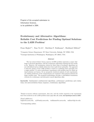
The paper expands on our work as reported in [15] and is organized as follows. Section 2briefly introduces two very different LABS solvers and the termination criteria that we applyto both, Section 3 defines the experimental set up that remains identical for both solvers,Section 4 summarizes the asymptotic performance of both solvers under termination criterion ‘A’ for L 47, Section 5 summarizes the predictions and the asymptotic performanceof the LABS solver of choice under termination criterion ‘B’ for L 47, Section 6 addressesfew questions that arise in view of the reported experimental results, Section 7 outlinesconclusions and future work.2LABS Solvers and Termination CriteriaWe introduce two LABS solvers at a level that will support a thorough one-on-one comparative analysis for both solvers. Evolutionary search (ES) techniques introduced in [16, 17]provide the background for the ES-solver that has been devised and optimized explicitlyfor the LABS problem [10]. Our alternative LABS solver, the KL-solver, is based on principles introduced in the classical graph partitioning paper by Kernighan and Lin [18] andsubsequently adapted to hypercube embedding [19, 20].2.1ES SolverEvolutionary strategies (ES) in its standard form start with an initial parent population ofλ binary strings, each of length L, and generated at random. Then µ children strings aregenerated, each by selecting a parent at random and applying a randomly chosen mutationoperation to it. From the µ children strings, one selects the λ best individuals, which formthe next parent population. The process is repeated until a termination criterion is met.Termination criteria are discussed later in this section. Militzer et al. [10] developed anovel mutation operator that appears to work particularly well for the LABS problem. Aflowchart view of the ES-solver as it traces the LABS problem landscape (for L 7) isshown in Figure 2. Clearly, with a single decision point, its ‘control structure’ at the levelshown is very simple – compared to the control structure at the same level for the KL-solver,to be discussed shortly.The main objectives of showing the traces below the ES flowchart are the following: (1)even for L 7, the energy cost (or fitness) function can vary two-orders of magnitude; (2)for choices of λ 3 and and µ 5, and running the solver for 4 generations (a total of 23samples) returns a local optimum solution with the energy cost of 7; (3) for choices of λ 3and and µ 5, and running the solver for 9 generations (a total of 48 samples) returns aglobal optimum solution with the cost of 3. Of course, the choice of the ES parameters inthis example is for simplicity of illustration only; we discuss the actual values used in thesection that follows.2.2KL SolverOur implementation of the KL solver samples the LABS cost function in a sequence ofwell-defined moves, starting from a randomly chosen initial binary string and evaluating thedistance-1 neighborhood of this string (flipping 1-bit at a time). We mark the bit for whichthe cost function was minimum and now repeat the process of evaluating the distance-1neighborhood, but now only with respect to the bits that are left unmarked. After the last4
Evolutionary strategy (ES) solver: key procedures and decisionsSolving the LABS problem of length L 7:(a) four generations of population samples finda local optimum cost of 7.Here, λ 3, µ 5 and total samples 3 4 5 23.cost function100101samples . 0generations .8162432404856(b) nine generations of population samples finda global optimum cost of 3.Here, λ 3, µ 5 and total samples 3 9 5 48.cost function100101samples . 0generations .8162432404856Figure 2: A flowchart view of the ES-solver as it traces the LABS problem landscape.5
Kernighan-Lin (KL) solver: key procedures and decisionsSolving the LABS problem of length L 7:(a) two sweeps of three move set samples terminate ata local optimum cost of 7. Here, restarts 0.Total samples 1 2 (7 6 5) 37.cost function100101samples . 0moves .sweeps .8162432404856(b) three sweeps of three move set samples terminate ata global optimum cost of 3. Here, restarts 1.Total samples 1 3 (7 6 5) 55.cost function100101samples . 0moves .sweeps .8162432404856Figure 3: A flowchart view of the KL-solver as it traces the LABS problem landscape.6
marking of the bits, we have evaluated L (L 1)/2 samples. We use the ‘best string’ fromthis search as the new starting point for the new sweep of distance-1 move set (after firstunmarking all of the bits). These sweeps are terminated once a new sweep produces a ‘beststring’ that is not better than the one saved from the previous sweep. At this point, theprocess is repeated with a new randomly selected string until a termination criterion is met.Termination criteria are discussed later in this section. A flowchart view of the KL-solver asit traces the LABS problem landscape (for L 7) is shown in Figure 3. Clearly, with threedecision points, the ‘control structure’ at the level shown is not as simple when compared tothe control structure at the same level for the ES-solver discussed earlier. For more detailsabout the KL-solver algorithm, see the Appendix.The main objectives of showing the traces below the KL flowchart are the following: (1) evenfor L 7, the energy cost (or fitness) function can vary two-orders of magnitude; (2) unlikefor ES, no user judgment is required to set-up the parameters that govern the selection ofstrings. For simplicity of illustration only, we make the decision that ‘all bits have beenmarked’ at the value of 7 7/2 4, so that each sweep contains only (7 6 5) 18samples. Here, we terminate after 0 restarts (a total of 37 samples) and return a localoptimum solution with the energy cost of 7; (3) Similarly to (2) above, we terminate after1 restart (a total of 55 samples) and return a global optimum solution with the energy costof 3.2.3Termination CriteriaThe simplest termination criterion in a stochastic search solver is the maxium time duration (timeout) of the experimental run from a given starting point. Such criterion isplatform-dependent. However, even if the two LABS solvers such as ES-solver and KLsolver described above are being executed on the same platform under the same timeoutlimit, we may learn very little about what factors may account for the significant differencein the observed performance of the two solvers. Note also that that the flow-chart level, thecombinatorial metrics decide the termination for each solver are different: the maximumnumber of generations (ES) versus the maximum number of restarts (KL). However, if wecount the number of samples, i.e. cost function evaluations performed by each solver, we dohave a metric that is common to both. Experiment show that samples correlate perfectlywith runtime (in seconds) of either solver.To improve the efficiency and the reliability of the solver selection process, we organize theexperiments under two termination criteria [14]: Termination criterion ‘A’ (for L 47). Use the known LABS minimum value for a givenL to terminate a local search algorithm when the optimal sequence is found for thefirst time. Variables recorded during this search include, at the minimum, runtimeand samples (the number of cost function evaluations) that are required to find theoptimum. Both are random variables for which we find statistics so we can deduce theprobability of success, Psucc , of finding the LABS minimum value, given the runtimeor samples constraints. Termination criterion ‘B’ (for L 47). Develop a predictor model based on results underTermination A to predict, for a given value of L, the required runtime and/or requiredsamples for which the solver must be allowed to run in order to find the global minimumwith the probability of success Psucc . The value of required samples must be used asthe termination criterion ‘B’ if experiments are executed on a platform different fromthe one used under the termination criterion ‘A’.7
Of course, we will run only the ‘best-of-the-two’ from KL-solver and ES-solver under thetermination B (for the given value of L).We summarize the details of experimental set-up in the next section. In particular, wedemonstrate that experiments under the termination criterion ‘A’ lead to a number ofimportant insights about the asymptotic and statistical performance of each solver.3Experimental SetupThe experimental testbed we use is outlined in Figure 4. Each experiment is initialized witha unique random seed from the file randomTriplets that contains three random integers oneach line, making the testbed environment cross-platform consistent for any LABS solverthat uses the standard IEEE random generator. Under the criterion ‘A’, the termination ofeach execution is controlled by the known optimum value stored in the file knownOptima,available at [6].Data of most interest generated by these experiments are runtime (seconds, platformspecific) and samples (total number of samples to evaluate the cost function, platformindependent). These two random variables are closely correlated and, not surprisingly, bothwill have exponential distribution for both ES and KL solver.1 While the exponential distribution of runtime or samples implies significant variability as illustrated in Figure 4, thevariability is also predictable – shown by the close fit of observed and theoretical distributions. For example, if we allow the KL solver to search for the optimum sequence of lengthL 34 for 3,088,247 samples (from any randomly choosen initial sequence), the probabilityof finding the optimum is 0.632. However, if we increase the search limit to 4*3,088,247samples or 8*3,088,247 samples, the probability increases to 0.981 or 0.999 respectively.The parameters used for all ES-solver experiments are based on settings evaluated as ‘bestoverall’ in [10]: λ 10 and µ 3 L. The single parameter used in KL-solver experimentsis bits-to-mark L/2. This is different from a default value of bits-to-mark L since weobserved no significant improvement (with respect to the LABS problem) if we marked allbits of the move set as defined in Figure 3.Thus, before starting the experiments with the two solvers, we made every effort not toviolate the “Pet Pieve 10. Hand-tuned algorithm parameters” that concludes with arecommended rule as follows [22]:If different parameter settings are to be used for different instances, the adjustment process must be well-defined and algorithmic, the adjustment must bedescribed in the paper, and the time for the adjustment must be included in allreported running times.We analyze the statistical performance of each solver in the next section.1 Exponential distribution of runtime has been observed not only for stochastic solvers in different contexts [21], but also within a unified framework for stochastic and branch-and-bound solvers applied to SATproblem instances [13]. Distributions other than exponential have also been observed in a number of relatedexperiments with several solvers [13].8
Experiments under termination ‘A’Create LABSbed as a LABS-problem specific testbed environment, simplerthan but similar to SATbed [23]. We consider (1) primary input filesrandomTriplets and knownOptima, (2) user-specified parameters L, solverList,nExperiments, (3) a solver encapsulator SolverEncap A( L, randomTriplets,knownOptima, solverList, nExperiments ) that returns rawData(solver , L),and (4) GetStats( rawData(solver , L) ) that returns statsData(solver , L).Invoke SolverEncap A to return a tabular report rawData(solver , L) for eachsolver and each L, with data columns under labels such as instanceNum,runtime, samples, solution.The number of rows is determined bynExperiments. For the same value of L, each experiment represents an equivalent problem instance, initialized by the LABS solver with a different randomseed triple from the file randomTriplets.solvability function (128 experiments)Invoke GetStats to return various statistics for random variables in each datacolumn in rawData(solver , L), including characterization of underlying distributions and the respective solvability functions [23]. As shown below, thenumber of samples (or function evaluations) required by the KL solver to findthe optimum solution for L 34 for each of the 128 experiments has exponential distribution and can vary dramatically. At best, an optimum solution isfound with 43,354 samples; at worst with 13,322,800 samples; with a median,mean and standard deviation of 2,11,5035 and 3,088,247 and 3,006,546 samples, respectively. The runtime mean value, specific to our platform (a LinuxPC with 266 MHz processor), is 6.60 seconds. Hyperlinks to complete rawand statistical results of experiments such as illustrated here, covering severalsolvers, and values of L up to 64 can be found on the newly created LABSbedhome page [24].1observed0.80.6PP succsucc0.632Psucc 1 - exp(-x / mean)wherex KL-samplesmean 3,088,247 (samples)0.40.200.0E 02.0E 64.0E 66.0E 68.0E 61.0E 71.2E 71.4E 7KL-samples to find optima for L 34 (128 experiments)Figure 4: Experimental flow under termination ’A’ (for any solver).4LABS Solver ComparisonsTo capture the asymptotic performance of the ES and KL solver under the termination‘A’ with statistical significance, we performed 128 experiments with each solver for eachvalue of L in the range of 10 L 47. Similarly to Figure 4, we observe for each Lan exponential distribution of runtime and samples for both solvers. Also, we observe9
exponential distribution for generations (ES solver) and restarts (KL solver).2 . However,with 128 trials the distribution of the reported means for each of these random variablesis near-normal due to the law of large numbers. Also with 128 trials, two means withcomparable standard deviation will pass a standard t-test for equivalence, at confidencelevel of 95%, as long as their ratios are bounded by 4/3 from above and 3/4s from below.In other words, after 128 independent experiments, we shall declare two LABS solvers suchas ES and KL to have significantly different performance only if the ratio of their meansexceeds 4/3 or is less than 3/4. For example, in Figure 4 we report for the value of L 34,the mean number of samples as 2,925,765 (ES solver) and – slightly better than the meannumber of samples 3,088,427 (KL solver). A t-test declares both means to be equivalent,and a χ2 -test declares both distributions to be equivalent.Comparison with a single value of L is not sufficient; we rely on the asymptotic analysis foraverages and ratios of averages based on 128 experiments for consecutive values of L 10to L 47 for both KL and ES solvers. As shown in Figure 5, we pair data reported bythe two solvers in terms of average samples, average runtime (in seconds), and the samplingefficiency defined as the ratio of the average number of samples to the average runtime.For each set of data we also show a regression line that nominally predicts the asympoticbehavior of each solver beyond the value of L 47:3ES samplesES runtimeES efficiencyKL samplesKL runtimeKL ictorpredictor 5.558E 1 1.370L 7.108E 4 1.397L 7.819E 4 0.981L 1.553E 1 1.423L 1.287E 5 1.463L 1.206E 6 0.973L(3)(4)(5)(6)(7)(8)Note however, that not all mean values for L 47 we report are actually on a given regressionline. For example, for the the ES-solver, we observe data points up to a factor of 2.0 aboveand 1.7 below the nominal ES samples predictor – until we reach the value of L 43. At thisvalue, we record a nearly 14-fold increase above the nominal ES samples predictor. Also,there is a reduction by a factor of 4.3 at L 46. Such variability is statistically significantas it clearly exceeds the [3/4, 4/3] bounds expected due to statistical variability alone. Asour detailed analysis in the next section suggests, the variability of the solver may be dueto two factors: (1) significant change of LABS problem landscape with change of L sincethe number of optimal solutions may vary significantly as illustrated in Table 1, and (2)partial mismatch of ES-solver parameters for the given value of L. Additional consecutivedata points are needed to more completely characterize the asymptotic performance of theES-solver; its performance variability may or may not exceed the variability demonstratedfor the KL-solver up to the value of L 64 in the section that follows.For the KL-solver, we observe data points up to a factor of 4.0 above and 3.6 below thenominal KL samples predictor – uniformly across the observed range. Again, such variationsby far exceed the expected statistical variations of the mean values. However, as shown inFigure 5, the sampling efficiency for the KL-solver is subject to noticeably smaller variationsthan the sampling efficiency for the ES-solver. We thus conjecture that the variabilityobserved for the KL-solver is mostly due to the variability of the LABS problem landscapewith change of L.2 Weremind the reader that when we observe that distribution is exponential, mean standard deviationthe consecutive values of L 20 to L 47 are used in the least-square fit to each data set. Datapoints for the ES-solver for L 50, 54, 58 are shown for illustration only.3 Only10
1E 10KL and ES total samples1.553E 1*1.423 L1E 91E 81E 75.558E 1 *1.370 L1E 6KL-samples (O(1.423 L))ES-samples (O(1.370 L))1E 51E 4ES-samples2025303540455055606570LABS length (L) vs KL and ES total samplesKL and ES runtime (seconds)1E 67.108E-4 *1.397 L1E 51E 41E 31E 21E 1KL-runtime (O(1.463 L))1E 0ES-runtime (O(1.397 L))1.287E-5 *1.463 L1E-11E-22025303540ES-runtime455055606570LABS length (L) vs KL and ES runtime (seconds)KL "sampling efficiency"8E 5se(L) 1.206E 6 * (0.973) LKL-Samples/Second (O(0.973 L))2E 520253035404550556065LABS length (L) vs KL "sampling efficiency" (se)70ES "sampling efficiency"6E 4se(L) 7.819E 4 * (0.981) LES-Samples/Second (O(0.981 L))ES-Samples/Second2E 42025303540455055606570LABS length (L) vs ES "sampling efficiency" (se)Figure 5: Asymptotic comparisons of ES and KL solvers.11
Asymptotically, the nominal performance of the ES-solver appears better: there is a crossoverof the samples predictors at L 34 and the runtime predictors at L 88. However, thesecrossovers are not well-defined due to the demonstrated variability and most importantly,there is a significant difference in the sampling efficiency between the two solvers; for L 34the average runtimes are 6.60 and 74.5 seconds for KL and ES, respectively. A significantimprovement of the sampling efficiency of the ES solver is needed to make it competitive,for L 88, with the current version of the KL solver.Experiments as report here were executed on 266 MHz workstation under Linux. Thecurrent platform is clearly unsuitable for experiments at L 88 even with the faster-of-thetwo solvers. For L 77, the projected runtime (using 1.552e-8*1.419L for the KL-solver) is0.94 years; if the processor performance would increase tenfold, it would still take 1.1 yearsto complete similar runs for L 84. What is needed is a LABS solver with both (1) runtimecomplexity significantly better than O(1.419L ) and (2) constant factor significantly betterthan 1.552e-8 relative to our 266 MHz platform.However, as presented in the next section, we can demonstrate the reliability of the costpredictor under the termination ‘B’ for the KL-solver in the range of 48 L 64 andslightly beyond.5Cost Predictions under Termination ‘B’We ask the question: ‘How long should the KL solver run in order to find the optimum fora given L with a certain probability of success Psucc ?’ We find the answer by analyzing theasymptotic behavior of either runtime, samples or restarts of the KL solver under terminationcriterion ‘A’. An example of restarts data is shown in the top part of Figure 6. The averagevalues of restarts are based on 128 experiments for consecutive values of L 20 to L 47.Also shown are three regression lines derived from the observed data for L 47 and datapoints as predicted by the respective regression lines for values of L 47:nominal restarts predictorupper bound restarts predictorlower bound restarts predictor 0.1351 1.331L0.6754 1.331L0.0270 1.331L(9)(10)(11)According to the nominal restarts predictor in (9), the number of required restarts to find theoptimum with Psucc 0.632 for L 48, 60, and 64, is 123,851 or 3,832,423 or 12,031,820,respectively. However, not all average restarts reported by the KL-solver are ‘on the line’that corresponds to the nominal restarts predictor. In fact, the maximum deviations fromthe nominal predictions for required restarts for the range of 20 L 47 are very significant:for L 26 the prediction is far too conservative (229 restarts predicted, 64 observed, a ratioof 3.59), for L 41 the prediction is far too optimistic (67,375 restarts observed, 16,726predicted, a ratio of 4.03). Such variations by far exceed the expected statistical variabilityof the observed mean values of restarts: the 95% confidence intervals for the observed meanvalues are [52 . 77] for L 26 and [55,527 . 79,222] for L 41, respectively. Theempirical upper bound restarts predictor in equation (10) simply multiplies the nominalrestarts predictor by a factor of 5 which is based both on the worst-case ratio of 4.03 and theobserved confidence interval for mean restarts at L 41. Using the upper bound restartspredictor, the number of required restarts for L 41 has the value of 81,380. Similarly, theempirical lower bound restarts predictor divides the nominal restarts predictor by a factorof 5. Clearly, such bounds may need to be adjusted for larger values of L when moreexperimental data becomes available.12
(a) restarts predictions for the termination criterion ‘B’restarts predictor ub (O(1.331 L))restarts predictor nom (O(1.331 L))restarts predictor lb (O(1.331 L))KL termination predictors and runtime hours1E 9restarts observed (O(1.331 L))1E 8runtime hours (O(1.419 L))1E 7restarts predictor ub 0.6754 * 1.331 L1E 61E 51E 4restarts predictor nom 0.1351 * 1.331 L1E 31E 21E 1hours 1.552E-8 * 1.419 L1E 01E-12025303540455055606570LABS length (L) vs KL-termination predictors & observed hours(b) summary of experiments based on predictions 188[6]197[6]205[6]218[
a single method: (1) solver performance experiments with problem sizes for which op-timal solutions are known, (2) an asymptotic statistical analysis of such experiments, (3) reliable predictions of the computational cost required to find optimal solutions for larger problem sizes. The proposed methodology provides a well-defined termination