Transcription
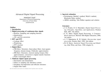
1Advanced Digital Signal ProcessingAbdellatif Zaidi †Department of Electrical EngineeringUniversity of Notre Dameazaidi@nd.eduOutline:1. Introduction2. Digital processing of continuous-time signals Retition: Sampling and sampling theorem Quantization AD- and DA-conversion3. DFT and FFT Leakage effect Windowing FFT structure4. Digital filters FIR-filters: Structures, linear phase filters, least-squaresfrequency domain design, Chebyshev approximation IIR-filters: Structures, classical analog lowpass filterapproximations, conversion to digital transfer functions Finite word-length effects5. Multirate digital signal processing Decimation and interpolation Filters in sampling rate alteration systems Polyphase decomposition and efficient structures Digital filter banks6. Spectral estimation Periodogram, Bartlett’s method, Welch’s method,Blackman-Tukey method ARMA modeling, Yule-Walker equation and solutionLiterature J. G. Proakis, D. G. Manolakis: Digital Signal Processing: Principles, Algorithms, and Applications, PrenticeHall, 2007, 4th edition S. K. Mitra: Digital Signal Processing: A ComputerBased Approach, McGraw Hill Higher Education, 2006,3rd edition A. V. Oppenheim, R. W. Schafer: Discrete-time signalprocessing, Prentice Hall, 1999, 2nd edition M. H. Hayes: Statistical Signal Processing and Modeling, John Wiley and Sons, 1996 (chapter 6).Parts of this textbook have been realized in close collaboration with Dr. Joerg Kliewer whom I warmly thank.2
– Numerical integration and differentiation– Determination of mean value, correlation, p.d.f., . . .1. Introduction1.1 Signals, systems and signal processingWhat does “Digital Signal Processing” mean?Signal: Physical quantity that varies with time, space or any otherindependent variable Mathematically: Function of one or more independentvariables, s1(t) 5 t, s2(t) 20 t2 Examples: Temperature over time t, brightness (luminance) ofan image over (x, y), pressure of a sound wave over (x, y, z)or (x, y, z, t)Speech signal:Amplitude 1x 1040.500.10.20.30.4t [s] 0.50.6Digital signal processing: Processing of signals by digital means(software and/or hardware)Includes: Conversion from the analog to the digital domain and back(physical signals are analog) Mathematical specification of the processing operations Algorithm: method or set of rules for implementing the systemby a program that performs the corresponding mathematicaloperations Emphasis on computationally efficient algorithms, which arefast and easily implemented. 0.5 1 Properties of the system (e.g. linear/nonlinear) determine theproperties of the whole processing operation System: Definition also includes:– software realizations of operations on a signal, whichare carried out on a digital computer ( softwareimplementation of the system)– digital hardware realizations (logic circuits) configuredsuch that they are able to perform the processing operation,or– most general definition: a combination of both0.7Signal Processing: Passing the signal through a system Examples:– Modification of the signal (filtering, interpolation, noisereduction, equalization, . . .)– Prediction, transformation to another domain (e.g. Fouriertransform)34
Basic elements of a digital signal processing system1.2 Digital signal processors (DSPs)Analog signal processing: Programmable microprocessor (more flexibility), or hardwireddigital processor (ASIC, application specific integrated circuit)(faster, ogoutputsignalOften programmable DSPs (simply called ”DSPs”) are used forevaluation purposes, for prototypes and for complex algorithms:Digital signal processing:(A/D: Analog-to-digital, D/A: signalD/AconverterAnalogoutputsignal Fixed-point processors: Twos-complement number representation. Floating-point processors: Floating point number representation (as for example used in PC processors)Why has digital signal processing become so popular?Overview over some available DSP processors see next page.Digital signal processing has many advantages compared toanalog processing:Performance example: 256-point complex exitygenerallyunlimited(costs, complexity precision)without problemslowgenerally erally limited (costsincrease drastically withrequired precision)problematichigherωdmin ωamin , ωdmax ωamaxexactly realizableapproximately realizablerealizablestrong limitations(from [Evaluating DSP Processor Performance, Berkeley Design Technology, Inc., 2000])56
Some currently available DSP processors and their properties (2006):ManufacturerFamilyArithmeticDatawidth (bits)BDTImark2000(TM)Coreclock speedUnit priceqty. 10000Analog 10n/a500146091301470160 MHz200 MHz750 MHz600 MHz275 MHz80 MHz300 MHz500 MHz40 MHz160 MHz300 MHz1 GHz300 MHz 11-26 5-15 5-32 131-205 4-47 3-12 13-35 77-184 2-8 3-54 4-17 15-208 12-31FreescaleTexas-Instuments78
92. Digital Processing of Continuous-Time SignalsDigital signal processing system from above is refined:Anti-aliasinglowpass filterSample-andhold circuitA/DLowpass reconstruction filterSample-andhold circuitD/ADigital signalprocessor2.1 Sampling Generation of discrete-time signals from continuous-timesignalsIdeal samplingIdeally sampled signal xs(t) obtained by multiplication of thecontinuous-time signal xc(t) with the periodic impulse trains(t) Xn δ(t nT ),where δ(t) is the unit impulse function and T the samplingperiod:xs(t) xc(t) · Xn Xn δ(t nT )xc(nT ) δ(t nT )(2.1)(2.2)10
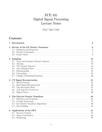
we finally have for the Fourier transform of xs(t)(”sifting property” of the impulse function)xc (t)(a)Xs(jΩ) ts(t)(b)(lengths of Dirac deltas correspond to their weighting) 1 XXc(j(Ω kΩs)).T k (2.4) Periodically repeated copies of Xs(jΩ)/T , shifted by integermultiples of the sampling frequency1Xc (jΩ)t0T2T3T4T(a)15T.xs (t)Ω(lengths of Dirac deltas correspond to their weighting)ΩN ΩN(c)S(jΩ).0T2T3T4T2πT(b)t5TΩ 3ΩsHow does the Fourier transform F {xs(t)} Xs(jΩ) looklike? 2Ωs ΩsΩs02Ωs3ΩsΩs2Ωs(Ωs ΩN )3Ωs2π6πXs (jΩ)1T(c)Fourier transform of an impulse train:Ω 2π Xs(t) S(jΩ) δ(Ω kΩs)T k 3Ωs. 2Ωs Ωs ΩNΩN(2.3) 6π 4π 2π04π.ωω ΩTXs (jΩ)Ωs 2π/T : sampling frequency in radians/s.Writing (2.1) in the Fourier domain,(d) Aliasing1TΩXs(jΩ) 1Xc(jΩ) S(jΩ),2πΩs 2Ωs(Ωs ΩN )1112
(a) Fourier transform of a bandlimited continuous-time inputsignal Xc(jΩ), highest frequency is ΩN(b) Fourier transform of the Dirac impulse train(c) Result of the convolution S(jΩ) Xc(jΩ). It is evident thatwhenΩs ΩN ΩN or Ωs 2ΩN(2.5)the replicas of Xc(jΩ) do not overlap. xc(t) can be recovered with an ideal lowpass filter!Representation with the discrete (normalized) frequencyω ΩT 2πf T (f frequency in Hz) for the discrete signal xc (nT ) x(n)with F {x(n)} X(ejω ), F {·} denoting the Fourier transform fordiscrete-time aperiodic signals (DTFT)Nonideal sampling Modeling the sampling operation with the Dirac impulse trainis not a feasible model in real life, since we always need a finiteamount of time for acquiring a signal sample.Nonideally sampled signal xn(t) obtained by multiplication of acontinuous-time signal xc(t) with a periodic rectangular windowfunction an(t): xn(t) xc(t) · an(t) wherean(t) a0(t) n δ(t n T ) Xn (2.8)rect(t) sinc(Ω/2),sinc(x) : sin(x)/x1tTTFourier transform of an(t):Fourier transform of the rectangular time window in (2.7) (seeproperties of the Fourier transform)A0(jΩ) F {a0(t)} α T · sinc(ΩαT /2) · e X(2.7)a 0 (t )(d) If (2.5) does not hold, i.e. if Ωs 2ΩN , the copies ofXc(jΩ) overlap and the signal xc(t) cannot be recovered bylowpass filtering. The distortions in the gray shaded areas arecalled aliasing distortions or simply aliasing.Also in (c):a0(t) denotes the rectangular prototype window: t αT /2a0(t) rectαT(0 for t 1/2with rect(t) : 1 for t 1/2a0(t nT )(2.6)13 jΩαT /2(2.9)Fourier transform of an(t) in (2.6) (analog to (2.3)):An(jΩ) A0(jΩ) · 2πα X 2π Xδ(Ω kΩs)T k sinc(kΩsα T /2) e jkΩs αT /2δ(Ω kΩs)k 2πα Xsinc(kπα) e jkπαδ(Ω kΩs)k (2.10)14
Sincexn(t) xc(t) an(t) Xn(jΩ) 1(Xc(jΩ) An(jΩ))2πSolution: Sampling is performed by a sample-and-hold (S/H)circuitwe finally have by inserting (2.10)Xn(jΩ) α Xsinc(kπα) e jkπαk Xc(j(Ω kΩs)).(2.11)From (2.11) we can deduce the following: Compared to the result in the ideal sampling case (cp. (2.4))here each repeated spectrum at the center frequency kΩs isweighted with the term sinc(kπα) e jkπα. The energy Xn(jΩ) 2 is proportional α2: This isproblematic since in order to approximate the ideal case wewould like to choose the parameter α as small as possible.(from [Proakis, Manolakis, 1996])(a) Basic elements of an A/D converter, (b) time-domain response of an idealS/H circuit The goal is to continously sample the input signal and to holdthat value constant as long as it takes for the A/D converter toobtain its digital representation. Ideal S/H circuit introduces no distortion and can be modeledas an ideal sampler. Drawbacks for the nonideal sampling case can be avoided(all results for the ideal case hold here as well).1516
Then, with the definition of the rect(·) function in (2.8) we have2.2 Sampling TheoremReconstruction of an ideally sampled signal by ideal lowpassfiltering:s(t) Pδ(t nT )n (a)xc (t)Hr (jΩ)xs (t)(d)Xc (jΩ)(b)xc(t) Hr (jΩ)xr (t)THr (jΩ) T rect(Ω/Ωs) hr (t) sinc(Ωst/2).(2.14)Combining (2.13), (2.14), and (2.2) yieldsΩN Ωc (Ωs ΩN )1 n Ω Ωc ΩcΩ ΩN(e)Xs (jΩ)1 1T(c) 2Ωs Ωs ΩN ΩNΩNΩs2Ωs(Ωs ΩN )ΩNIn order to get the input signal xc(t) back after reconstruction,i.e. Xr (jΩ) Xc(jΩ), the conditionsΩN Ωs2andΩN Ωc (Ωs ΩN ) X(2.12)Z xc(nT ) sincδ(τ nT ) sinc 1Ωs(t nT )21Ωs(t τ )2 dτ dτ1Ωs(t τ )2 .Sampling theorem:Every bandlimited continuous-time signal xc(t) withΩN Ωs/2 can be uniquely recovered from its samplesxc(nT ) according toxc(t) Xn have both to be satisfied. Then,Xc(jΩ) Xr (jΩ) Xs(jΩ) · Hr (jΩ)xc(nT )n ΩΩ Xxc(nT ) δ(τ nT ) sincn Xr (jΩ)ΩNZ X xc(nT ) sinc 1Ωs(t nT )2 .(2.15)Remarks: xc(t) xr (t) xs(t) hr (t). (2.13) Eq. (2.15) is called the ideal interpolation formula, and thesinc-function is named ideal interpolation functionWe now choose the cutoff frequency Ωc of the lowpass filter asΩc Ωs/2 (satisfies both inequalities in (2.12)).1718
Reconstruction of a continuous-time signal using idealinterpolation: S/H circuit serves as a ”deglitcher”:Output of the D/A converter is held constant at the previousoutput value until the new sample at the D/A output reachessteady state(from [Proakis, Manolakis, 1996])Anti-aliasing lowpass filtering:In order to avoid aliasing, the continuous-time input signal has tobe bandlimited by means of an anti-aliasing lowpass-filter withcut-off frequency Ωc Ωs/2 prior to sampling, such that thesampling theorem is satisfied.2.3 Reconstruction with sample-and-hold circuitIn practice, a reconstruction is carried out by combining a D/Aconverter with a S/H circuit, followed by a lowpass reconstruction(smoothing) filterdigitalinput signalD/AS/Hh0 (t)x0 (t)Lowpasshr (t)(from [Proakis, Manolakis, 1996])xDA (t) D/A converter accepts electrical signals that correspond tobinary words as input, and delivers an output voltage or currentbeing proportional to the value of the binary word for everyclock interval nT Often, the application on an input code word yields ahigh-amplitude transient at the output of the D/A converter(”glitch”)19Analysis:The S/H circuit has the impulse response t T /2h0(t) rectT(2.16)which leads to a frequency responseH0(jΩ) T · sinc(ΩT /2) · e jΩT /2(2.17)20
No sharp cutoff frequency response characteristics wehave undesirable frequency components (above Ωs/2), whichcan be removed by passing x0(t) through a lowpassreconstruction filter hr (t). This operation is equivalentto smoothing the staircase-like signal x0(t) after the S/Hoperation.(a) Xs (jΩ) 1T Xc (jΩ) Ω Ωs0 When we now suppose that the reconstruction filter hr (t) isan ideal lowpass with cutoff frequency Ωc Ωs/2 and anamplification of one, the only distortion in the reconstructedsignal xDA(t) is due to the S/H operation:Ωs2ΩsT sinc(ΩT /2)(b)TΩ Ωs0Ωs2ΩsΩs2Ωs X0 (jΩ) (c) XDA(jΩ) Xc(jΩ) · sinc(ΩT /2) 1T1(2.18)Ω Ωs Xc(jΩ) denotes the magnitude spectrum for the idealreconstruction case.0 Hr (jΩ) (d)1 Additional distortion when the reconstruction filter is not ideal(as in real life!) Distortion due to the sinc-function may be corrected by prebiasing the frequency response of the reconstruction filterΩc Ωs /2Ω Ωs Ωc0ΩcΩs XDA (jΩ) (e)1Spectral interpretation of the reconstruction process (see next page):(a) Magnitude frequency response of the ideally sampled continuous-timesignalΩ Ωs0Ωs(b) Frequency response of the S/H circuit (phase factor e jΩT /2 omitted)(c) Magnitude frequency response after the S/H circuit(d) Magnitude frequency response: lowpass reconstruction filter(e) Magnitude frequency response of the reconstructed continuous-time signal2122
2.4 QuantizationConversion carried out by an A/D converter involves quantizationof the sampled input signal xs(nT ) and the encoding of theresulting binary representation Example: midtreat quantizer with L 8 levels and rangeR 8 4 d1 3 2 0 2 3 x1 d2 x2 d3 x3 d4 x4 d5 x5 d6 x6 d7 x7 d8 x8d9 Amplitude Quantization is a nonlinear and noninvertible process whichrealizes the mappingxs(nT ) x(n) xk I,(2.19)where the amplitude xk is taken from a finite alphabet I . Signal amplitude range is divided into L intervals In using theL 1 decision levels d1, d2, . . . , dL 1:In {dk x(n) dk 1},Quantization Decisionlevelslevelsd3 x3 d4 x4 d5k 1, 2, . . . , LRange R of quantizer Quantization error e(n) with respect to the unquantizedsignal (2.21) e(n) 22If the dynamic range of the input signal (xmax xmin) islarger than the range of the quantizer, the samples exceedingthe quantizer range are clipped, which leads to e(n) /2. Quantization characteristic function for a midtreat quantizerwith L 8:Ikdk xk dk 1Amplitude Mapping in (2.19) is denoted as x̂(n) Q[x(n)] Uniform or linear quantizers with constant quantization stepsize are very often used in signal processing applications: xk 1 xk const.,for all k 1, 2, . . . , L 1(2.20) Midtreat quantizer: Zero is assigned a quantization levelMidrise quantizer: Zero is assigned a decision level(from [Proakis, Manolakis, 1996])2324
significant bit (LSB), has the valueCodingThe coding process in an A/D converter assigns a binary numberto each quantization level.b With a wordlength of b bits we can represent 2 L binarynumbers, which yieldsb log2(L).(2.22) The step size or the resolution of the A/D converter is given as R2bwith the range R of the quantizer.x β0 b 1Xβℓ 2 ℓ(2.24)ℓ 1 Number representation has no influence on the performance ofthe quantization process!Performance degradations in practical A/D converters:(2.23) Commonly used bipolar codes:(from [Proakis, Manolakis, 1996]) Two’s complement representation is used in most fixedpoint DSPs: A b-bit binary fraction [β0β1β2 . . . βb 1], β0denoting the most significant bit (MSB) and βb 1 the least25(from [Proakis, Manolakis, 1996])26
Quantization errorsQuantization error is modeled as noise, which is added to theunquantized signal:Actual systemx(n)QuantizerQ(x(n))where σx2 denotes the signal power and σe2 the power of thequantization noise.Quantization noise is assumed to be uniformly distributed in therange ( /2, /2):p(e)x̂(n)1 e(n)Mathematical modelx(n) 2x̂(n) x(n) e(n)e 2 Zero mean, and a variance ofAssumptions: The quantization error e(n) is uniformly distributed over the range 2 e(n) 2 . The error sequence e(n) is modeled as a stationary whitenoise sequence. The error sequence e(n) is uncorrelated with the signalsequence x(n).2σeZ /21 e p(e) de /2Effect of the quantization error or quantization noise on theresulting signal x̂(n) can be evaluated in terms of the signal-tonoise ratio (SNR) in Decibels (dB)SNR : 10 log10!,(2.25) 2e de 12 /2 /22(2.26)2σe Assumptions do not hold in general, but they are fairly wellsatisfied for large quantizer wordlengths b.ZInserting (2.23) into (2.26) yields The signal sequence is assumed to have zero mean.σx2σe222 2b R2,12(2.27)and by using this in (2.25) we obtain!!12 22b σx2 10 log10SNR 10 log10R2 R 6.02 b 10.8 20 log10dB.(2.28)σx {z}σx2σe2( )Term ( ) in (2.28):2728
σx root-mean-square (RMS) amplitude of the signal v(t) σx to small decreasing SNR Furthermore (not directly from ( )): σx to large range Ris exceeded2.5 Analog-to-digital converter realizationsFlash A/D converter Signal amplitude has to be carefully matched to the range ofthe A/D converterFor music and speech a good choice is σx R/4. Then the SNRof a b-bit quantizer can be approximately determined asSNR 6.02 b 1.25 dB.Analogcomparator:(2.29)Each additional bit in the quantizer increases the signal-to-noiseratio by 6 dB!(from [Mitra, 2000], N b: resolution in bits) Analog input voltage VA is simultaneously compared with aset of 2b 1 separated reference voltage levels by means of aset of 2b 1 analog comparators locations of the comparatorcircuits indicate range of the input voltage.Examples:Narrowband speech: b 8 Bit SNR 46.9 dBMusic (CD): b 16 Bit SNR 95.1 dBMusic (Studio): b 24 Bit SNR 143.2 dB All output bits are developed simultaneously very fastconversion Hardware requirements increase exponentially with anincrease in resolution Flash converters are used for low-resultion (b 8 bit) andhigh-speed conversion applications.Serial-to-parallel A/D convertersHere, two b/2-bit flash converters in a serial-parallelconfiguration are used to reduce the hardware complextityat the expense of a slightly higher conversion time2930
Subranging A/D converter:approximation in the shift register is converted into an (analog)reference voltage VD by D/A conversion (binary representation[β0β1 . . . βk βk 1 . . . βb 1], βk {0, 1} k): Case 1: Reference voltage VD VA increase the binarynumber by setting both the k-th bit and the (k 1)-th bit to 1 Case 2: Reference voltage VD VA decrease the binarynumber by setting the k-th bit to 0 and the (k 1)-th bit to 1(from [Mitra, 2000], N b: resolution in bits) High resolution and fairly high speed at moderate costs, widelyused in digital signal processing applicationsRipple A/D converter:Oversampling sigma-delta A/D converter, to be discussed in Section 5. . .2.6 Digital-to-analog converter realizationsWeighted-resistor D/A converter(from [Mitra, 2000], N b: resolution in bits)Advantage of both structures: Always one converter is idle whilethe other one is operating Only one b/2-bit converter is necessaryNSucessive approximation A/D converterN1210(from [Mitra, 2000], N b: resolution in bits)Output Vo of the D/A converter is given byVo N 1Xℓ 0(from [Mitra, 2000], N b: resolution in bits)Iterative approach: At the k-th step of the iteration the binary31ℓ2 βℓ(2NRLVR 1)RL 1VR : reference voltageFull-scale output voltage Vo,F S is obtained when βℓ 1 for allℓ 0, . . . , N 1:32
Vo,F S(2N 1)RLN NVR VR , since (2 1)RL 1(2 1)RL 1Disadvantage: For high resolutions the spread of the resistorvalues becomes very large3. DFT and FFT3.1 DFT and signal processingDefinition DFT from Signals and Systems:Resistor-ladder D/A converterDFT: v(n) VN (k) 0123N2N1ℓ2 βℓℓ 0(3.2)3.1.1 Linear and circular convolutionVRRL· N 12(RL R) 2Linear convolution of two sequences v1(n) and v2(n), n ZZ:In practice, often 2RL R, and thus, the full-scale outputvoltage Vo,F S is given asVo,F S(3.1)n 0with WN : e j2π/N , N : number of DFT points R–2R ladder D/A converter, most widely used in practice.Output Vo of the D/A converter:Vo knv(n) WNN 11 X knVN (k) WNIDFT: VN (k) v(n) N k 0(from [Mitra, 2000], N b: resolution in bits)N 1XN 1Xyl (n) v1(n) v2(n) v2(n) v1(n) (2N 1) VR2N Xk v1(k) v2(n k) Xk v2(k) v1(n k) (3.3)Circular convolution of two periodic sequences v1(n) andv2(n), n {0, . . . , N1,2 1} with the same periodN1 N2 N and n0 ZZ:Oversampling sigma-delta D/A converter, to be discussed in Section 5. . .3334
Substitution of the DFT definition in (3.1) for v1(n) and v2(n):yc(n) v1(n) v2(n) v2(n) v1(n) n0 N 1Xk n0v1(k) v2(n k) n0 N 1Xk n0v2(k) v1(n k)(3.4)"## " N 1N 1 N 1X1 X X knklkmy(n) v2(l)WN WNv1(m)WNN k 0 m 0l 0#"N 1N 1N 1XX1 X k(n m l)WNv1(m)v2(l) N m 0k 0l 0(3.7)We also use the symbolNinstead of .DFT and circular convolutionInverse transform of a finite-length sequence v(n),n, k 0, . . . , N 1:v(n) VN (k) v(n) v(n λN )(3.5) DFT of a finite-length sequence and its periodic extension isidentical!Circular convolution property (n, k 0, . . . , N 1)(v1(n) and v2(n) denote finite-length sequences):y(n) v1(n)Nv2(n) Y (k) V1N (k) · V2N (k)Term in brackets: Summation over the unit circle(N 1XNfor l n m λN, λ ZZj2πk(n m l)/Ne 0otherwisek 0(3.8)Substituting (3.8) into (3.7) yields the desired relationy(n) Proof:v1(k)k 0 Xλ v2(n k λN ){z} : v2 ((n k))N (periodic extension) (3.6)N 1XN 1Xk 0v1(k)v2((n k))N v1(n)N(3.9)v2(n)N 11 X knIDFT of Y (k): y(n) Y (k)WNN k 0N 11 X knV1N (k)V2N (k)WN N k 03536
Example: Circular convolution y(n) v1(n)Noperation for linear filtering is linear convolution. How canthis be achieved by means of the DFT?v2(n):v2 (n)Given: Finite-length sequences v1(n) with length N1 and v2(n)with length N2n0 Linear convolution:Nv1 (n) δ(n 1)y(n) k 0n0NkNv2 ((1 k))N , k 0, . . . , N 1, n 1k0This result can be summarized as follows:The circular convolution of two sequences v1(n) with length N1and v2(n) with length N2 leads to the same result as the linearconvolution v1(n) v2(n) when the lengths of v1(n) and v2(n)are increased to N N1 N2 1 points by zero padding.NN v2 (n)y(n) v1 (n) n0v1(k) v2(n k)Length of the convolution result y(n): N1 N2 1 Frequency domain equivalent: Y (ejω ) V1(ejω ) V2(ejω ) In order to represent the sequence y(n) uniquely in thefrequency domain by samples of its spectrum Y (ejω ), thenumber of samples must be equal or exceed N1 N2 1 DFT of size N N1 N2 1 is required. Then, the DFT of the linear convolution y(n) v1(n) v2(n) is Y (k) V1(k) · V2(k), k 0, . . . , N 1.v2 ((0 k))N , k 0, . . . , N 1, n 00N1 1XN3.1.2 Use of the DFT in linear filtering Filtering operation can also be carried out in the frequencydomain using the DFT attractive since fast algorithms (fastFourier transforms) exist DFT only realizes circular convolution, however, the desired37Other interpretation:Circular convolution as linearconvolution with aliasingIDFT leads to periodic sequence in the time-domain: P y(n λN ) n 0, . . . , N 1,yp(n) λ 0otherwise38
with Y (k) DFTN {y(n)} DFTN {yp(n)}3.1.3 Filtering of long data sequences For N N1 N2 1: Circular convolution equivalent tolinear convolution followed by time domain aliasingExample:nN1 N20N1Overlap-add method1. Input signal is segmented into separate blocks:vν (n) v(n νN1), n {0, 1, . . . , N1 1}, ν ZZ.2. Zero-padding for the signal blocks vν (n) ṽν (n) and theimpulse response h(n) h̃(n) to the length N N1 N2 1.Input signal can be reconstructed according tox1 (n) x2 (n)N1 N2 61Filtering of a long input signal v(n) with the finite impulseresponse h(n) of length N2y(n) x1 (n) x2 (n)n02N1 1N1v(n) ν y(n N1 ), N1 6N1N1Yν (k) Ṽν (k) · H̃(k),y(n N1 ), N1 6N1x1 (n) N x2 (n)N1 N2 6nN1 N20N1y(n) N x2 (n)x1 (n) N 12 Xν n0k 0, . . . , N 1.4. The N -point IDFT yields data blocks that are free fromaliasing due to the zero-padding in step 2.5. Since each input data block vν (n) is terminated with N N1zeros the last N N1 points from each output block yν (n)must be overlapped and added to the first N N1 points of thesucceeding block (linearity property of convolution):n0 N1ṽν (n νN1)since ṽν (n) 0 for n N1 1, . . . , N .3. The two N -point DFTs are multiplied together to formn0 Xyν (n νN1) Overlap-add method2N1 13940
Linear FIR (finite impulse response) filtering by the overlap-addmethod:Input signal:x̂0 (n)LL5. In order to avoid the loss of samples due to aliasing the lastN N1 samples are saved and appended at the beginning ofthe next block. The processing is started by setting the firstN N1 samples of the first block to zero.11000011N N1 zerosx̂1 (n)11000011Linear FIR filtering by the overlap-save method:Input signal:N N1 zerosx̂2 (n)110000110011001111000011N N1 zerosOutput signal:y0 (n)1100001100110011N N1 samplesadded togethery1 (n)Lx0 (n)N N1 zeros1100001100110011N N1 samplesadded togethery2 (n)11000011L1100001100110011N LL4. Since the input signal block is of length N the first N N1points are corrupted by aliasing and must be discarded. Thelast N2 N N1 1 samples in yν (n) are exactly the sameas the result from linear convolution.x1 (n)Output signal:Overlap-save method1. Input signal is segmented into by N N1 samples overlappingblocks:vν (n) v(n νN1), n {0, 1, . . . , N 1}, ν ZZ.2. Zero-padding of the filter impulse response h(n) h̃(n) tothe length N N1 N2 1.11000011L1100001100110011x2 (n)11000011y0 (n)DiscardN N1 samples11000011y1 (n)DiscardN N1 samples11000011y2 (n)DiscardN N1 samples3. The two N -point DFTs are multiplied together to formYν (k) Vν (k) · H̃(k), k 0, . . . , N 1.Nore computationally efficient than linear convolution? Yes, incombination with very efficient algorithms for DFT computation.4142
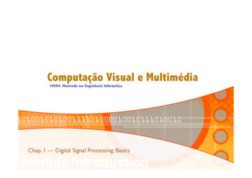
We finally have3.1.4 Frequency analysis of stationary signalsLeakage effectjωi1 hjωjωV (e ) W (e )2πi1hj(ω ω0 )j(ω ω0 )W (e) W (e) 2V̂ (e ) Spectral analysis of an analog signal v(t): Antialiasing lowpass filtering and sampling with Ωs 2Ωb,Ωb denoting the cut-off frequency of the signal For practical purposes (delay, complexity): Limitation of thesignal duration to the time interval T0 L T (L: number ofsamples under consideration, T : sampling interval)(3.13)Nagnitude frequency response V̂ (ejω ) for L 25:Limitation to a signal duration of T0 can be modeled asmultiplication of the sampled input signal v(n) with a rectangularwindow w(n)(from [Proakis, Nanolakis, 1996])v̂(n) v(n) w(n) with w(n) (1 for 0 n L 1,0 otherwise.(3.10)Suppose that the input sequence just consists of a single sinusoid,that is v(n) cos(ω0n). The Fourier transform isjωV (e ) π(δ(ω ω0) δ(ω ω0)).(3.11)W (e ) L 1Xn 0e jωnFirst zero crossing of W (ejω ) at ωz 2π/L: The larger the number of sampling points L (and thus also thewidth of the rectangular window) the smaller becomes ωz (andthus also the main lobe of the frequency response). Decreasing the frequency resolution leads to an increaseof the time resolution and vice versa (duality of time andfrequency domain).For the window w(n) the Fourier transform can be obtained asjωWindowed spectrum V̂ (ejω ) is not localized to one frequency,instead it is spread out over the whole frequency range spectral leaking1 e jωL jω(L 1)/2 sin(ωL/2) . e jω1 esin(ω/2)(3.12)43In practice we use the DFT in order to obtain a sampledrepresentation of the spectrum according to V̂ (ejωk ),k 0, . . . , N 1.44
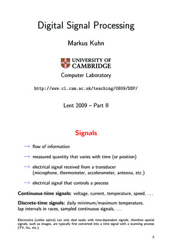
Special case: IfN L and ω0 2πν,Nν 0, . . . , N 1then the Fourier transform is exactly zero at the sampledfrequencies ωk , except for k ν .Example: (N 64, n 0, . . . , N 1, rectangular windoww(n)) 2ππ2πn , v1(n) cos5 nv0(n) cos 5NNNv0(n) cos(2π/N 5 n)v1(n) cos((2π/N 5 π/N) n)110.50.500ωk k2π/N except for k 5, since ω0 is exactly an integermultiple of 2π/N periodic repetition of v0(n) leads to a pure cosinesequence Right hand side: slight increase of ω0 6 ν2π/N for ν ZZ V̂1(ejωk ) 6 0 for ωk k2π/N , periodic repetition isnot a cosine sequence anymoreWindowing and different window functionsWindowing not only distorts the spectral estimate due to leakageeffects, it also reduces the spectral resolution.Consider a sequence of two frequency componentsv(n) cos(ω1n) cos(ω2n) with the Fourier transformjωV (e ) 1hj(ω ω1 )j(ω ω2 )W (e) W (e) 2 W (e 0.5 1 0.50204060 10nDFT(v0(n) w(n)), rect. window10.80.80.60.60.40.40.20.201020k4030001020 W (ej(ω ω2 ))iwhere W (ejω ) is the Fourier transform of the rectangularwindow from (3.12).60nDFT(v1(n) w(n)), rect. window1020j(ω ω1 )) 2π/L ω1 ω2 : Two maxima, main lobes for both windowspectra W (ej(ω ω1)) and W (ej(ω ω2)) can be separated ω1 ω2 2π/L: Correct values of the spectral samples,but main lobes cannot be separated anymore ω1 ω2 2π/L: Nain lobes of W (ej(ω ω1)) andW (ej(ω ω2)) overlap30k Left hand side: V̂0(ejωk ) V0(ejωk ) W (ejωk ) 0 for45 Ability to resolve spectral lines of different frequencies islimited by the main lobe width, which also depends on the lengthof the window impulse response L.46
Example: Magnitude frequency response V (ejω ) forv(n) cos(ω0n) cos(ω1n) cos(ω2n)window, specified as(3.14)with ω0 0.2 π , ω1 0.22 π , ω2 0.6 π and (a) L 25,(b) L 50, (c) L 100wHan(n) h 1 1 cos2 02πL 1 n ifor 0 n L 1,otherwise.(3.15)Nagnitude frequency response V̂ (ejω ) from (3.13), whereW (ejω )
2. Digital Processing of Continuous-Time Signals Digital signal processing system from above is refined: Digital signal processor A/D D/A Sample-and-struction filter hold circuit Lowpass recon-lowpass filter Anti-aliasing Sample-and-hold circuit 2.1 Sampling Generation of discrete-time signals from continuous-time signals Ideal sampling