Transcription
ECE 301: Signals and SystemsCourse NotesProf. Shreyas SundaramSchool of Electrical and Computer EngineeringPurdue University
ii
AcknowledgmentsThese notes very closely follow the book: Signals and Systems, 2nd edition, byAlan V. Oppenheim, Alan S. Willsky with S. Hamid Nawab. Parts of the notesare also drawn from Linear Systems and Signals by B. P. Lathi A Course in Digital Signal Processing by Boaz Porat Calculus for Engineers by Donald TrimI claim credit for all typos and mistakes in the notes.The LATEX template for The Not So Short Introduction to LATEX 2ε by T. Oetikeret al. was used to typeset portions of these notes.Shreyas SundaramPurdue University
iv
Contents1 Introduction11.1Signals and Systems . . . . . . . . . . . . . . . . . . . . . . . . .11.2Outline of This Course . . . . . . . . . . . . . . . . . . . . . . . .42 Properties of Signals and Systems52.1Signal Energy and Power . . . . . . . . . . . . . . . . . . . . . .52.2Transformations of Signals . . . . . . . . . . . . . . . . . . . . . .72.3Periodic, Even and Odd Signals . . . . . . . . . . . . . . . . . . .72.4Exponential and Sinusoidal Signals . . . . . . . . . . . . . . . . .82.4.1Continuous-Time Complex Exponential Signals . . . . . .82.4.2Discrete-Time Complex Exponential Signals . . . . . . . .9Impulse and Step Functions . . . . . . . . . . . . . . . . . . . . .122.5.1Discrete-Time . . . . . . . . . . . . . . . . . . . . . . . . .122.5.2Continuous-Time . . . . . . . . . . . . . . . . . . . . . . .13Properties of Systems . . . . . . . . . . . . . . . . . . . . . . . .142.6.1Interconnections of Systems . . . . . . . . . . . . . . . . .142.6.2Properties of Systems . . . . . . . . . . . . . . . . . . . .152.52.63 Analysis of Linear Time-Invariant Systems213.1Discrete-Time LTI Systems . . . . . . . . . . . . . . . . . . . . .213.2Continuous-Time LTI Systems . . . . . . . . . . . . . . . . . . .233.3Properties of Linear Time-Invariant Systems . . . . . . . . . . . .243.3.1The Commutative Property . . . . . . . . . . . . . . . . .243.3.2The Distributive Property . . . . . . . . . . . . . . . . . .243.3.3The Associative Property . . . . . . . . . . . . . . . . . .25
viCONTENTS3.43.53.3.4Memoryless LTI Systems . . . . . . . . . . . . . . . . . .263.3.5Invertibility of LTI Systems . . . . . . . . . . . . . . . . .273.3.6Causality of LTI Systems . . . . . . . . . . . . . . . . . .283.3.7Stability of LTI Systems . . . . . . . . . . . . . . . . . . .283.3.8Step Response of LTI Systems . . . . . . . . . . . . . . .29Differential and Difference Equation Models for Causal LTI Systems 303.4.1Linear Constant-Coefficient Differential Equations . . . .313.4.2Linear Constant Coefficient Difference Equations . . . . .33Block Diagram Representations of Linear Differential and Difference Equations . . . . . . . . . . . . . . . . . . . . . . . . . . . .354 Fourier Series Representation of Periodic Signals374.1Applying Complex Exponentials to LTI Systems . . . . . . . . .4.2Fourier Series Representation of Continuous-Time Periodic Signals 404.3Calculating the Fourier Series Coefficients . . . . . . . . . . . . .424.3.1A Vector Analogy for the Fourier Series . . . . . . . . . .44Properties of Continuous-Time Fourier Series . . . . . . . . . . .484.4.1Linearity . . . . . . . . . . . . . . . . . . . . . . . . . . .494.4.2Time Shifting . . . . . . . . . . . . . . . . . . . . . . . . .494.4.3Time Reversal . . . . . . . . . . . . . . . . . . . . . . . .504.4.4Time Scaling . . . . . . . . . . . . . . . . . . . . . . . . .504.4.5Multiplication . . . . . . . . . . . . . . . . . . . . . . . . .514.4.6Parseval’s Theorem . . . . . . . . . . . . . . . . . . . . . .52Fourier Series for Discrete-Time Periodic Signals . . . . . . . . .524.5.1Finding the Discrete-Time Fourier Series Coefficients . . .534.5.2Properties of the Discrete-Time Fourier Series . . . . . . .554.44.55 The Continuous-Time Fourier Transform5.13759The Fourier Transform . . . . . . . . . . . . . . . . . . . . . . . .595.1.1Existence of Fourier Transform . . . . . . . . . . . . . . .625.2Fourier Transform of Periodic Signals . . . . . . . . . . . . . . . .635.3Properties of the Continuous-Time Fourier Transform . . . . . .645.3.1Linearity . . . . . . . . . . . . . . . . . . . . . . . . . . .655.3.2Time-Shifting . . . . . . . . . . . . . . . . . . . . . . . . .65
CONTENTSvii5.3.3Conjugation . . . . . . . . . . . . . . . . . . . . . . . . . .655.3.4Differentiation . . . . . . . . . . . . . . . . . . . . . . . .665.3.5Time and Frequency Scaling. . . . . . . . . . . . . . . .675.3.6Duality . . . . . . . . . . . . . . . . . . . . . . . . . . . .675.3.7Parseval’s Theorem . . . . . . . . . . . . . . . . . . . . . .685.3.8Convolution . . . . . . . . . . . . . . . . . . . . . . . . . .685.3.9Multiplication . . . . . . . . . . . . . . . . . . . . . . . . .726 The Discrete-Time Fourier Transform756.1The Discrete-Time Fourier Transform . . . . . . . . . . . . . . .756.2The Fourier Transform of Discrete-Time Periodic Signals . . . . .786.3Properties of the Discrete-Time Fourier Transform . . . . . . . .796.3.1Periodicity . . . . . . . . . . . . . . . . . . . . . . . . . .796.3.2Linearity . . . . . . . . . . . . . . . . . . . . . . . . . . .796.3.3Time and Frequency Shifting . . . . . . . . . . . . . . . .796.3.4First Order Differences . . . . . . . . . . . . . . . . . . . .806.3.5Conjugation . . . . . . . . . . . . . . . . . . . . . . . . . .806.3.6Time-Reversal . . . . . . . . . . . . . . . . . . . . . . . .806.3.7Time Expansion . . . . . . . . . . . . . . . . . . . . . . .816.3.8Differentiation in Frequency . . . . . . . . . . . . . . . . .826.3.9Parseval’s Theorem . . . . . . . . . . . . . . . . . . . . . .826.3.10 Convolution . . . . . . . . . . . . . . . . . . . . . . . . . .826.3.11 Multiplication . . . . . . . . . . . . . . . . . . . . . . . . .837 Sampling877.1The Sampling Theorem . . . . . . . . . . . . . . . . . . . . . . .877.2Reconstruction of a Signal From Its Samples. . . . . . . . . . .897.2.1Zero-Order Hold . . . . . . . . . . . . . . . . . . . . . . .897.2.2First-Order Hold . . . . . . . . . . . . . . . . . . . . . . .907.3Undersampling and Aliasing . . . . . . . . . . . . . . . . . . . . .907.4Discrete-Time Processing of Continuous-Time Signals . . . . . .91
viiiCONTENTS8 The Laplace Transform958.1The Laplace Transform . . . . . . . . . . . . . . . . . . . . . . .958.2The Region of Convergence . . . . . . . . . . . . . . . . . . . . .988.3The Inverse Laplace Transform . . . . . . . . . . . . . . . . . . . 1018.3.18.4Partial Fraction Expansion . . . . . . . . . . . . . . . . . 102Some Properties of the Laplace Transform . . . . . . . . . . . . . 1038.4.1Convolution . . . . . . . . . . . . . . . . . . . . . . . . . . 1048.4.2Differentiation . . . . . . . . . . . . . . . . . . . . . . . . 1048.4.3Integration . . . . . . . . . . . . . . . . . . . . . . . . . . 1048.5Finding the Ouput of an LTI System via Laplace Transforms . . 1058.6Finding the Impulse Response of a Differential Equation via LaplaceTransforms . . . . . . . . . . . . . . . . . . . . . . . . . . . . . . 106
Chapter 1Introduction1.1Signals and SystemsLoosely speaking, signals represent information or data about some phenomenonof interest. This is a very broad definition, and accordingly, signals can be foundin every aspect of the world around us.For the purposes of this course, a system is an abstract object that accepts inputsignals and produces output signals in response.InputSystemOutputFigure 1.1: An abstract representation of a system.Examples of systems and associated signals: Electrical circuits: voltages, currents, temperature,. Mechanical systems: speeds, displacement, pressure, temperature, volume, . Chemical and biological systems: concentrations of cells and reactants,neuronal activity, cardiac signals, . Environmental systems: chemical composition of atmosphere, wind patterns, surface and atmospheric temperatures, pollution levels, . Economic systems: stock prices, unemployment rate, tax rate, interestrate, GDP, . Social systems: opinions, gossip, online sentiment, political polls,. Audio/visual systems: music, speech recordings, images, video, .
2Introduction Computer systems: Internet traffic, user input, .From a mathematical perspective, signals can be regarded as functions of oneor more independent variables. For example, the voltage across a capacitor inan electrical circuit is a function of time. A static monochromatic image canbe viewed as a function of two variables: an x-coordinate and a y-coordinate,where the value of the function indicates the brightness of the pixel at that(x, y) coordinate. A video is a sequence of images, and thus can be viewedas a function of three variables: an x-coordinate, a y-coordinate and a timeinstant. Chemical concentrations in the earth’s atmosphere can also be viewedas functions of space and time.In this course, we will primarily be focusing on signals that are functions of asingle independent variable (typically taken to be time). Based on the examplesabove, we see that this class of signals can be further decomposed into twosubclasses: A continuous-time signal is a function of the form f (t), where t rangesover all real numbers (i.e., t R). A discrete-time signal is a function of the form f [n], where n takes on onlya discrete set of values (e.g., n Z).Note that we use square brackets to denote discrete-time signals, and roundbrackets to denote continuous-time signals. Examples of continuous-time signals often include physical quantities, such as electrical currents, atmosphericconcentrations and phenomena, vehicle movements, etc. Examples of discretetime signals include the closing prices of stocks at the end of each day, populationdemographics as measured by census studies, and the sequence of frames in adigital video. One can obtain discrete-time signals by sampling continuous-timesignals (i.e., by selecting only the values of the continuous-time signal at certainintervals).Just as with signals, we can consider continuous-time systems and discretetime systems. Examples of the former include atmospheric, physical, electricaland biological systems, where the quantities of interest change continuously overtime. Examples of discrete-time systems include communication and computingsystems, where transmissions or operations are performed in scheduled timeslots. With the advent of ubiquitous sensors and computing technology, thelast few decades have seen a move towards hybrid systems consisting of bothcontinuous-time and discrete-time subsystems – for example, digital controllersand actuators interacting with physical processes and infrastructure. We willnot delve into such hybrid systems in this course, but will instead focus onsystems that are entirely either in the continuous-time or discrete-time domain.The term dynamical system loosely refers to any system that has an internalstate and some dynamics (i.e., a rule specifying how the state evolves in time).
1.1 Signals and Systems3This description applies to a very large class of systems, including individual vehicles, biological, economic and social systems, industrial manufacturing plants,electrical power grid, the state of a computer system, etc. The presence of dynamics implies that the behavior of the system cannot be entirely arbitrary; thetemporal behavior of the system’s state and outputs can be predicted to someextent by an appropriate model of the system.Example 1.1. Consider a simple model of a car in motion. Let the speed ofthe car at any time t be given by v(t). One of the inputs to the system is theacceleration a(t), applied by the throttle. From basic physics, the evolution ofthe speed is given bydv a(t).(1.1)dtThe quantity v(t) is the state of the system, and equation (1.1) specifies thedynamics. There is a speedometer on the car, which is a sensor that measuresthe speed. The value provided by the sensor is denoted by s(t) v(t), and thisis taken to be the output of the system.Much of scientific and engineering endeavor relies on gathering, manipulatingand understanding signals and systems across various domains. For example,in communication systems, the signal represents voice or data that must betransmitted from one location to another. These information signals are oftencorrupted en route by other noise signals, and thus the received signal mustbe processed in order to recover the original transmission. Similarly, social,physical and economic signals are of great value in trying to predict the currentand future state of the underlying systems. The field of signal processing studieshow to take given signals and extract desirable features from them, often viathe design of systems known as filters. The field of control systems focuseson designing certain systems (known as controllers) that measure the signalscoming from a given system and apply other input signals in order to makethe given system behave in an desirable manner. Typically, this is done via afeedback loop of the formDesiredOutputControlInput ControllerSystemOutputSensorFigure 1.2: Block Diagram of a feedback control system.Example 1.2 (Inverted Pendulum). Suppose we try to balance a stick verticallyin the palm of our hand. The sensor, controller and actuator in this exampleare our eyes, our brain, and our hand, respectively, which communicate usingsignals of various forms. This is an example of a feedback control system.
4Introduction1.2Outline of This CourseSince the concepts of signals and systems are prevalent across a wide variety ofdomains, we will not attempt to discuss each specific application in this course.Instead, we will deal with the underlying mathematical theory, analysis, anddesign of signals and systems. In this sense, it will be more mathematical thanother engineering courses, but will be different from other math courses in thatit will pull together various branches of mathematics for a particular purpose(i.e., to understand the nature of signals and systems).The main components of this course will be as follows. Signal and systems classifications: develop terminology and identify usefulproperties of signals and systems Time domain analysis of LTI systems: understand how the output of lineartime-invariant systems is related to the input Frequency domain analysis techniques and signal transformations (Fourier,Laplace, z-transforms): study methods to study signals and systems froma frequency domain perspective, gaining new ways to understand theirbehavior Sampling and Quantization: study ways to convert continuous-time signals into discrete-time signals, along with associated challengesThe material in this course will lay the foundations for future courses in controltheory (ECE 382, ECE 483), communication systems (ECE 440) and signalprocessing (ECE438, 445).
Chapter 2Properties of Signals andSystemsWe will now identify certain useful properties and classes of signals and systems.Recall that a continuous-time signal is denoted by f (t) (i.e., a function of thereal-valued variable t) and a discrete-time signal is denoted by f [n] (i.e., afunction of the integer-valued variable n). When drawing discrete-time signals,we will use a sequence of dots to indicate the discrete nature of the time variable.2.1Signal Energy and PowerSuppose that we consider a resistor in an electrical circuit, and let v(t) denotethe voltage signal across the resistor i(t) denote the current. From Ohm’s law,we know that v(t) i(t)R, where R is the resistance. The power dissipated bythe resistor is thenv 2 (t)p(t) v(t)i(t) i2 (t)R .RThus the power is a scaled multiple of the square of the voltage and currentsignals.Since the energy expended over a time-interval [t1 , t2 ] is given by the integral ofthe power dissipated per-unit-time over that interval, we haveZ t2Z t2Z1 t2 2E p(t)dt Ri2 (t)dt v (t)dt.R t1t1t1The average power dissipated over the time-interval [t1 , t2 ] is then111E t2 t1t2 t1 RZt2t1v 2 (t)dt Rt2 t1Zt2t1i2 (t)dt.
6Properties of Signals and SystemsWe will find it useful to discuss the energy and average power of any continuoustime or discrete-time signal. In particular, the energy of a general (potentiallycomplex-valued) continuous-time signal f (t) over a time-interval [t1 , t2 ] is defined asZ t2E[t1 ,t2 ] , f (t) 2 dt,t1where f (t) denotes the magnitude of the signal at time t.Similarly, the energy of a general (potentially complex-valued) discrete-timesignal f [n] over a time-interval [n1 , n2 ] is defined asE[n1 ,n2 ] ,n2X f [n] 2 .n n1Note that we are defining the energy of an arbitrary signal in the above way;this will end up being a convenient way to measure the “size” of a signal, andmay not actually correspond to any physical notion of energy.We will also often be interested in measuring the energy of a given signal overall time. In this case, we defineZ E , f (t) 2 dt for continuous-time signals, andE , X f [n] 2n for discrete-time signals. Note that the quantity E may not be finite.Similarly, we define the average power of a continuous-time signal asZ T1 f (t) 2 dt,P , limT 2T Tand for a discrete-time signal asNX1 f [n] 2 .N 2N 1P , limn NBased on the above definitions, we have three classes of signals: finite energy(E ), finite average power (P ), and those that have neither finiteenergy nor average power. An example of the first class is the signal f (t) e tfor t 0 and f (t) 0 for t 0. An example of the second class is f (t) 1 forall t R. An example of the third class is f (t) t for t 0. Note that anysignal that has finite energy will also have finite average power, sinceE 02Tfor continuous-time signals with finite energy, with an analogous characterization for discrete-time signals.P limT
2.2 Transformations of Signals2.27Transformations of SignalsThroughout the course, we will be interested in manipulating and transformingsignals into other forms. Here, we start by considering some very simple transformations involving the time variable. For the purposes of introducing thesetransformations, we will consider a continuous-time signal f (t) and a discretetime signal f [n].Time-shifting: Suppose we define another signal g(t) f (t t0 ), where t0 R.In other words, for every t R, the value of the signal g(t) at time t is the valueof the signal f (t) at time t t0 . If t0 0, then g(t) is a “forward-shifted” (ortime-delayed) version of f (t), and if t0 0, then g(t) is a time-advanced versionof f (t) (i.e., the features in f (t) appear earlier in time in g(t)). Similarly, for adiscrete-time signal f [n], one can define the time-shifted signal f [n n0 ], wheren0 is some integer.Time-reversal: Consider the signal g(t) f ( t). This represents a reversalof the function f (t) in time. Similarly, f [ n] represents a time-reversed versionof the signal f [n].Time-scaling: Define the signal g(t) f (αt), where α is some real number.When 0 α 1, this represents a stretching of f (t), and when α 1, thisrepresents a compression of f (t). If α 0, we get a time-reversed and stretched(or compressed) version of f (t). Analogous definitions hold for the discrete-timesignal f [n].The operations above can be combined to define signals of the form g(t) f (αt β), where α and β are real numbers. To draw the signal g(t), we shouldfirst apply the time-shift by β to f (t) and then apply the scaling α. To see why,define h(t) f (t β), and g(t) h(αt). Thus, we have g(t) f (αt β) asrequired. If we applied the operations in the other order, we would first get thesignal h(t) f (αt), and then g(t) h(t β) f (α(t β)) f (αt αβ). Inother words, the shift would be by αβ rather than β.Examples of these operations can be found in the textbook (OW), such asexample 1.1.2.3Periodic, Even and Odd SignalsA continuous-time signal f (t) is said to be periodic with period T if f (t) f (t T ) for all t R. Similarly, a discrete-time signal f [n] is periodic withperiod N if f [n] f [n N ] for all n Z. The fundamental period of a signalis the smallest period for which the signal is periodic.A signal is even if f (t) f ( t) for all t R (in continuous-time), or f [n] f [ n] for all n Z (in discrete-time). A signal is odd if f (t) f ( t) for allt R, or f [n] f [ n] for all n Z. Note that if a signal is odd, it mustnecessarily be zero at time 0 (since f (0) f (0)).
8Properties of Signals and SystemsGiven a signal f (t), define the signalse(t) 1(f (t) f ( t)) ,2o(t) 1(f (t) f ( t)) .2It is easy to verify that o(t) is an odd signal and e(t) is an even signal. Furthermore, x(t) e(t) o(t). Thus, any signal can be decomposed as a sum of aneven signal and an odd signal.2.42.4.1Exponential and Sinusoidal SignalsContinuous-Time Complex Exponential SignalsConsider a signal of the formf (t) Ceatwhere C and a are complex numbers. If both C and a are real, there are threepossible behaviors for this signal. If a 0, then the signal goes to zero ast , and if a 0, the signal goes to as t . For a 0, the signal isconstant.Now suppose f (t) ej(ω0 t φ) for some positive real number ω0 and real numberφ (this corresponds to C ejφ and a jω0 in the signal given above). We firstnote thatf (t T ) ej(ω0 (t T ) φ) ej(ω0 t φ) ejω0 T .If T is such that ω0 T is an integer multiple of 2π, we have ejω0 T 1 and thesignal is periodic with period T . Thus, the fundamental period of this signal isT0 2π.ω0Note that if ω0 0, then f (t) 1 and is thus periodic with any period. Thefundamental period is undefined in this case. Also note that f (t) e jω0 Tis also periodic with period T0 . The quantity ω0 is called the fundamentalfrequency of the signal.Note that periodic signals (other than the one that is zero for all time) haveinfinite energy, but finite average power. Specifically, letZ T0Ep f (t) 2 dt0be the energy of the signal over one period. The average power over that periodEis then Pp T0p , and since this extends over all time, this ends up being theaverage power of the signal as well. For example, for the signal f (t) ej(ω0 t φ) ,we haveZ TZ T11 f (t) 2 dt lim1dt 1.P limT 2T TT 2T T
2.4 Exponential and Sinusoidal Signals9Given a complex exponential with fundamental frequency ω0 , a harmonicallyrelated set of complex exponentials is a set of periodic exponentials of the formφk (t) ejkω0 t , k Z.In other words, it is the set of complex exponentials whose frequencies aremultiples of the fundamental frequency ω0 . Note that if ejω0 t is periodic withperiod T0 (i.e, ω0 T0 2πm for some integer m), then φk (t) is also periodic withperiod T0 for any k Z, sinceφk (t T0 ) ejkω0 (t T0 ) ejkω0 T0 ejkω0 t ejkm2π φk (t) φk (t).Although the signal f (t) given above is complex-valued in general, its real partand imaginary part are sinusoidal. To see this, use Euler’s formula to obtainAej(ω0 t φ) A cos(ω0 t φ) jA sin(ω0 t φ).Similarly, we can writeA cos(ω0 t φ) A j(ω0 t φ) A j(ω0 t φ)e e,22i.e., a sinusoid can be written as a sum of two complex exponential signals.Using the above, there are two main observations. First, continuous-time complex exponential signals are periodic for any ω0 R (the fundamental period is2πω0 for ω0 6 0 and undefined otherwise). Second, the larger ω0 gets, the smallerthe period gets.We will now look at discrete-time complex exponential signals and see that theabove two observations do not necessarily hold for such signals.2.4.2Discrete-Time Complex Exponential SignalsAs in the continuous-time case, a discrete-time complex exponential signal is ofthe formf [n] Ceanwhere C and a are general complex numbers. As before, let us focus on the casewhere C 1 and a jω0 for some ω0 R in order to gain some intuition, i.e.,f [n] ejω0 n .To see the differences in discrete-time signals from continuous-time signals, recall that a continuous-time complex exponential is always periodic for any ω0 .The first difference between discrete-time complex exponentials and continuoustime complex exponentials is that discrete-time complex exponentials are notnecessarily periodic. Specifically, consider the signal f [n] ejω0 n , and supposeit is periodic with some period N0 . Then by definition, it must be the case thatf [n N0 ] ejω0 (n N0 ) ejω0 n ejω0 N0 f [n]ejω0 N0 .
10Properties of Signals and SystemsDue to periodicity, we must have ejω0 N0 1, or equivalently, ω0 N0 2πk forsome integer k. However, N0 must be an integer, and thus we see that this canbe satisfied if and only of ω0 is a rational multiple of 2π. In other words, onlydiscrete-time complex exponentials whose frequencies are of the formω0 2πkNfor some integers k and N are periodic. The fundamental period N0 of a signalis the smallest nonnegative integer for which the signal is periodic. Thus, fordiscrete-time complex exponentials, we find the fundamental period by firstwritingkω0 2πNwhere k and N have no factors in common. The value of N in this representationis then the fundamental period.2π3πExample 2.1. Consider the signal f [n] ej 3 n ej 4 n . Since both of theexponentials have frequencies that are rational multiples of 2π, they are bothperiodic. For the first exponential, we have2π32π 1,3which cannot be reduced any further. Thus the fundamental period of the firstexponential is 3. Similarly, for the second exponential, we have3π42π 3.8Thus the fundamental period of the second exponential is 8. Thus f [n] is periodic with period 24 (the least common multiple of the periods of the twosignals).The same reasoning applies to sinusoids of the form f [n] cos(ω0 n). A necessary condition for this function to be periodic is that there are two positiveintegers n1 , n2 with n2 n1 such that f [n1 ] f [n2 ]. This is equivalent tocos(ω0 n1 ) cos(ω0 n2 ). Thus, we must either haveω0 n2 ω0 n1 2πkorω0 n2 ω0 n1 2πkfor some positive integer k. In either case, we see that ω0 has to be a rationalmultiple of 2π. In fact, when ω0 is not a rational multiple of 2π, the functioncos(ω0 n) never takes the same value twice for positive values of n.The second difference from continuous-time complex exponentials pertains tothe period of oscillation. Specifically, even for periodic discrete-time complex
2.4 Exponential and Sinusoidal Signals11exponentials, increasing the frequency does not necessarily make the periodsmaller. Consider the signal g[n] ej(ω0 2π)n , i.e., a complex exponential withfrequency ω0 2π. We haveg[n] ejω0 n ej2πn ejω0 n f [n],i.e., the discrete-time complex exponential with frequency ω0 2π is the sameas the discrete-time complex exponential with frequency ω0 , and thus they havethe same fundamental period. More generally, any two complex exponentialsignals whose frequencies differ by an integer multiple of 2π are, in fact, thesame signal.This shows that all of the unique complex exponential signals of the form ejω0 nhave frequencies that are confined to a region of length 2π. Typically, we willconsider this region to be 0 ω0 2π, or π ω0 π. Suppose we considerthe interval 0 ω0 2π. Note thatejω0 n cos(ω0 n) j sin(ω0 n).As ω0 increases from 0 to π, the frequencies of both the sinusoids increase.1 Forthose ω0 between 0 and π that are also rational multiples of π, the sampledsignals will be periodic, and their period will decrease as ω0 increases.Now suppose π ω0 2π. Consider the frequency 2π ω0 , which falls between0 and π. We haveej(2π ω0 )n e jω0 n cos(ω0 n) j sin(ω0 n).Since ejω0 n cos(ω0 n) j sin(ω0 n), the frequency of oscillation of the discretetime complex exponential with frequency ω0 is the same as the frequency ofoscillation of the discrete-time complex exponential with frequency 2π ω0 .Thus, as ω0 crosses π and moves towards 2π, the frequency of oscillation startsto decrease.To illustrate this, it is again instructive to consider the sinusoidal signals f [n] cos(ω0 n) for ω0 {0, π2 , π, 3π2 }. When ω0 0, the function is simply constant at1 (and thus its period is undefined). We see that the functions with ω0 π2 and2ω0 3π2 have the same period (in fact, they are exactly the same function).The following table shows the differences between continuous-time and discretetime signals.1 As we will see later in the course, the signals cos(ω n) and sin(ω n) correspond to00continuous-time signals of the form cos(ω0 t) and sin(ω0 t) that are sampled at 1 Hz. Whenω00 ω0 π, this sampling rate is above the Nyquist frequency π , and thus the sampledsignals will be an accurate representation of the underlying continuous-time signal.2 Note that cos(ω n) cos((2π ω )n) for any 0 ω π. The same is not true for000sin(ω0 n). In fact, one can show that for any two different frequencies 0 ω0 ω1 2π,sin(ω0 n) and sin(ω1 n) are different functions.
12Properties of Signals and Systemsejω0 tDistinct signals for different values of ω0Periodic for any ω0Fundamental period: undefined for2πotherwiseω0 0 and ω0Fundamental frequency ω0ejω0 nIdentical signals for values of ω0 separated by 2πkPeriodic only if ω0 2π Nfor some integers k and N 0.Fundamental period undefined for ω0 2πotherwise0 and k ω0Fundamental frequency ωk0As with continuous-time signals, for any period N , we define the harmonicfamily of discrete-time complex exponentials as2πφk [n] ejk N n , k Z.This is the set of all discrete-time complex exponentials that have a commonperiod N , and frequencies whose multiples of 2πN . This family will play a rolein our analysis later in the course.2.52.5.1Impulse and Step FunctionsDiscrete-TimeThe discrete-time unit impulse signal (or function) is defined as(0 if n 6 0δ[n] .1 if n 0The discrete-time unit step signal is defined as(0 if n 0.u[n] 1 if n 0Note that by the time-shifting property, we haveδ[n] u[n] u[n
These notes very closely follow the book: Signals and Systems, 2nd edition, by Alan V. Oppenheim, Alan S. Willsky with S. Hamid Nawab. Parts of the notes are also drawn from Linear Systems and Signals by B. P. Lathi A Course in Digital Signal Processing by Boaz Porat Calculus for Engineers by Donald Trim