Transcription
ACTIVE CALCULUS2015 EditionMatthew BoelkinsDavid AustinSteven Schlicker
2
Active Calculus2015 editionMatthew Boelkins, Lead Author and EditorDepartment of MathematicsGrand Valley State /boelkinm/David Austin, Contributing Authorhttp://merganser.math.gvsu.edu/david/Steven Schlicker, Contributing Authorhttp://faculty.gvsu.edu/schlicks/July 30, 2015
ii 2012-2015 BoelkinsThis work may be copied, distributed, and/or modified under the conditions of the Creative CommonsAttribution-NonCommercial-ShareAlike 3.0 Unported License.The work may be used for free by any party so long as attribution is given to the authors, that the work andits derivatives are used in the spirit of “share and share alike,” and that no party may sell this work or any ofits derivatives for profit, with the following exception: it is entirely acceptable for university bookstores to sellbound photocopied copies to students at their standard markup above the copying expense. Full details may be foundby sa/3.0/contacting Creative Commons, 444 Castro Street, Suite 900, Mountain View, California, 94041, USA.The Current Maintainer of this work is Matt Boelkins.First print edition:August 2014Boelkins, M.Austin, D. and Schlicker, S. –Orthogonal Publishing L3Cp. 549Includes illustrations, links to Java applets, and index.Cover photo: James Haefner Photography.ISBN 978-0-9898975-3-2
ContentsPreface1viiUnderstanding the Derivative11.1How do we measure velocity? . . . . . . . . . . . . . . . . . . . . . . . . .11.2The notion of limit . . . . . . . . . . . . . . . . . . . . . . . . . . . . . . .111.3The derivative of a function at a point . . . . . . . . . . . . . . . . . . . .221.4The derivative function . . . . . . . . . . . . . . . . . . . . . . . . . . . . .341.5Interpreting, estimating, and using the derivative . . . . . . . . . . . . . .431.6The second derivative . . . . . . . . . . . . . . . . . . . . . . . . . . . . . .521.7Limits, Continuity, and Differentiability . . . . . . . . . . . . . . . . . . . .651.8The Tangent Line Approximation . . . . . . . . . . . . . . . . . . . . . . .772 Computing Derivatives872.1Elementary derivative rules . . . . . . . . . . . . . . . . . . . . . . . . . . .872.2The sine and cosine functions . . . . . . . . . . . . . . . . . . . . . . . . .962.3The product and quotient rules . . . . . . . . . . . . . . . . . . . . . . . . 1022.4Derivatives of other trigonometric functions . . . . . . . . . . . . . . . . . 1132.5The chain rule . . . . . . . . . . . . . . . . . . . . . . . . . . . . . . . . . . 1192.6Derivatives of Inverse Functions . . . . . . . . . . . . . . . . . . . . . . . . 1292.7Derivatives of Functions Given Implicitly . . . . . . . . . . . . . . . . . . . 1402.8Using Derivatives to Evaluate Limits . . . . . . . . . . . . . . . . . . . . . . 1493 Using Derivatives3.1161Using derivatives to identify extreme values . . . . . . . . . . . . . . . . . 161iii
ivCONTENTS3.2Using derivatives to describe families of functions . . . . . . . . . . . . . . 1753.3Global Optimization . . . . . . . . . . . . . . . . . . . . . . . . . . . . . . . 1833.4Applied Optimization . . . . . . . . . . . . . . . . . . . . . . . . . . . . . . 1923.5Related Rates . . . . . . . . . . . . . . . . . . . . . . . . . . . . . . . . . . 1984 The Definite Integral4.1Determining distance traveled from velocity . . . . . . . . . . . . . . . . . 2094.2Riemann Sums . . . . . . . . . . . . . . . . . . . . . . . . . . . . . . . . . . 2234.3The Definite Integral . . . . . . . . . . . . . . . . . . . . . . . . . . . . . . 2364.4The Fundamental Theorem of Calculus . . . . . . . . . . . . . . . . . . . . 2525 Finding Antiderivatives and Evaluating Integrals2675.1Constructing Accurate Graphs of Antiderivatives . . . . . . . . . . . . . . 2675.2The Second Fundamental Theorem of Calculus . . . . . . . . . . . . . . . 2785.3Integration by Substitution . . . . . . . . . . . . . . . . . . . . . . . . . . . 2905.4Integration by Parts . . . . . . . . . . . . . . . . . . . . . . . . . . . . . . . 3015.5Other Options for Finding Algebraic Antiderivatives . . . . . . . . . . . . 3125.6Numerical Integration . . . . . . . . . . . . . . . . . . . . . . . . . . . . . . 3216 Using Definite Integrals72093356.1Using Definite Integrals to Find Area and Length . . . . . . . . . . . . . . 3356.2Using Definite Integrals to Find Volume . . . . . . . . . . . . . . . . . . . . 3456.3Density, Mass, and Center of Mass . . . . . . . . . . . . . . . . . . . . . . . 3566.4Physics Applications: Work, Force, and Pressure . . . . . . . . . . . . . . . 3676.5Improper Integrals . . . . . . . . . . . . . . . . . . . . . . . . . . . . . . . . 379Differential Equations3897.1An Introduction to Differential Equations . . . . . . . . . . . . . . . . . . . 3897.2Qualitative behavior of solutions to DEs . . . . . . . . . . . . . . . . . . . 4007.3Euler’s method . . . . . . . . . . . . . . . . . . . . . . . . . . . . . . . . . . 4117.4Separable differential equations . . . . . . . . . . . . . . . . . . . . . . . . 4217.5Modeling with differential equations . . . . . . . . . . . . . . . . . . . . . . 4297.6Population Growth and the Logistic Equation . . . . . . . . . . . . . . . . 437
CONTENTS8 Sequences and Seriesv4498.1Sequences . . . . . . . . . . . . . . . . . . . . . . . . . . . . . . . . . . . . 4498.2Geometric Series . . . . . . . . . . . . . . . . . . . . . . . . . . . . . . . . . 4588.3Series of Real Numbers . . . . . . . . . . . . . . . . . . . . . . . . . . . . . 4708.4Alternating Series . . . . . . . . . . . . . . . . . . . . . . . . . . . . . . . . 4888.5Taylor Polynomials and Taylor Series . . . . . . . . . . . . . . . . . . . . . 5038.6 Power Series . . . . . . . . . . . . . . . . . . . . . . . . . . . . . . . . . . . 520A A Short Table of Integrals533
viCONTENTS
PrefaceA free and open-source calculusSeveral fundamental ideas in calculus are more than 2000 years old. As a formalsubdiscipline of mathematics, calculus was first introduced and developed in the late 1600s,with key independent contributions from Sir Isaac Newton and Gottfried Wilhelm Leibniz.Mathematicians agree that the subject has been understood rigorously since the work ofAugustin Louis Cauchy and Karl Weierstrass in the mid 1800s when the field of modernanalysis was developed, in part to make sense of the infinitely small quantities on whichcalculus rests. Hence, as a body of knowledge calculus has been completely understoodby experts for at least 150 years. The discipline is one of our great human intellectualachievements: among many spectacular ideas, calculus models how objects fall underthe forces of gravity and wind resistance, explains how to compute areas and volumes ofinteresting shapes, enables us to work rigorously with infinitely small and infinitely largequantities, and connects the varying rates at which quantities change to the total changein the quantities themselves.While each author of a calculus textbook certainly offers her own creative perspectiveon the subject, it is hardly the case that many of the ideas she presents are new. Indeed, themathematics community broadly agrees on what the main ideas of calculus are, as well astheir justification and their importance; the core parts of nearly all calculus textbooks arevery similar. As such, it is our opinion that in the 21st century – an age where the internetpermits seamless and immediate transmission of information – no one should be requiredto purchase a calculus text to read, to use for a class, or to find a coherent collection ofproblems to solve. Calculus belongs to humankind, not any individual author or publishingcompany. Thus, a main purpose of this work is to present a new calculus text that is free.In addition, instructors who are looking for a calculus text should have the opportunity todownload the source files and make modifications that they see fit; thus this text is opensource. Since August 2013, Active Calculus has been endorsed by the American Institute ofMathematics and its Open Textbook Initiative: http://aimath.org/textbooks/.Because the text is free, any professor or student may use the electronic version of thetext for no charge. A .pdf copy of the text may be obtained by download fromhttp://gvsu.edu/s/xr,vii
viiiwhere the user will also find a link to a print-on-demand for purchasing a bound, softcoverversion for about 20. Other ancillary materials, such as WeBWorK .def files, an activitiesonly workbook, and sample computer laboratory activities are available upon direct requestto the author. Furthermore, because the text is open-source, any instructor may acquirethe full set of source files, again by request to the author at boelkinm@gvsu.edu. Thiswork is licensed under the Creative Commons Attribution-NonCommercial-ShareAlike 3.0Unported License. The graphicthat appears throughout the text shows that the work is licensed with the CreativeCommons, that the work may be used for free by any party so long as attribution is givento the author(s), that the work and its derivatives are used in the spirit of “share and sharealike,” and that no party may sell this work or any of its derivatives for profit, with thefollowing exception: it is entirely acceptable for university bookstores to sell bound photocopiedcopies of the activities workbook to students at their standard markup above the copying expense.Full details may be found by sa/3.0/or sending a letter to Creative Commons, 444 Castro Street, Suite 900, Mountain View,California, 94041, USA.Active Calculus: our goalsIn Active Calculus, we endeavor to actively engage students in learning the subject throughan activity-driven approach in which the vast majority of the examples are completed bystudents. Where many texts present a general theory of calculus followed by substantialcollections of worked examples, we instead pose problems or situations, consider possibilities, and then ask students to investigate and explore. Following key activities or examples,the presentation normally includes some overall perspective and a brief synopsis of generaltrends or properties, followed by formal statements of rules or theorems. While we oftenoffer plausibility arguments for such results, rarely do we include formal proofs. It is notthe intent of this text for the instructor or author to demonstrate to students that the ideasof calculus are coherent and true, but rather for students to encounter these ideas in asupportive, leading manner that enables them to begin to understand for themselves whycalculus is both coherent and true. This approach is consistent with the growing body ofscholarship that calls for students to be interactively engaged in class.
ixMoreover, this approach is consistent with the following goals: To have students engage in an active, inquiry-driven approach, where learners striveto construct solutions and approaches to ideas on their own, with appropriatesupport through questions posed, hints, and guidance from the instructor and text. To build in students intuition for why the main ideas in calculus are natural andtrue. Often, we do this through consideration of the instantaneous position andvelocity of a moving object, a scenario that is common and familiar. To challenge students to acquire deep, personal understanding of calculus throughreading the text and completing preview activities on their own, through working onactivities in small groups in class, and through doing substantial exercises outside ofclass time. To strengthen students’ written and oral communicating skills by having them writeabout and explain aloud the key ideas of calculus.Features of the TextInstructors and students alike will find several consistent features in the presentation,including: Motivating Questions. At the start of each section, we list 2-3 motivating questionsthat provide motivation for why the following material is of interest to us. One goalof each section is to answer each of the motivating questions. Preview Activities. Each section of the text begins with a short introduction,followed by a preview activity. This brief reading and the preview activity aredesigned to foreshadow the upcoming ideas in the remainder of the section; boththe reading and preview activity are intended to be accessible to students in advanceof class, and indeed to be completed by students before a day on which a particularsection is to be considered. Activities. A typical section in the text has three activities. These are designedto engage students in an inquiry-based style that encourages them to constructsolutions to key examples on their own, working individually or in small groups. Exercises. There are dozens of calculus texts with (collectively) tens of thousandsof exercises. Rather than repeat standard and routine exercises in this text, werecommend the use of WeBWorK with its access to the National Problem Libraryand around 20,000 calculus problems. In this text, there are approximately fourchallenging exercises per section. Almost every such exercise has multiple parts,requires the student to connect several key ideas, and expects that the student
xwill do at least a modest amount of writing to answer the questions and explaintheir findings. For instructors interested in a more conventional source of exercises,consider the freely available text by Gilbert Strang of MIT, available in .pdf formatfrom the MIT open courseware site via http://gvsu.edu/s/bh. Graphics. As much as possible, we strive to demonstrate key fundamental ideasvisually, and to encourage students to do the same. Throughout the text, we usefull-color1 graphics to exemplify and magnify key ideas, and to use this graphicalperspective alongside both numerical and algebraic representations of calculus. Links to Java Applets. Many of the ideas of calculus are best understood dynamically; java applets offer an often ideal format for investigations and demonstrations.Relying primarily on the work of David Austin of Grand Valley State Universityand Marc Renault of Shippensburg University, each of whom has developed a largelibrary of applets for calculus, we frequently point the reader (through active linksin the .pdf version of the text) to applets that are relevant for key ideas underconsideration. Summary of Key Ideas. Each section concludes with a summary of the key ideasencountered in the preceding section; this summary normally reflects responses tothe motivating questions that began the section.How to Use this TextThis text may be used as a stand-alone textbook for a standard first semester collegecalculus course or as a supplement to a more traditional text. Chapters 1-4 address thetypical topics for differential calculus, while Chapters 5-8 provide the standard topics ofintegral calculus, including a chapter on differential equations (Chapter 7) and on infiniteseries (Chapter 8).ElectronicallyBecause students and instructors alike have access to the book in .pdf format, there areseveral advantages to the text over a traditional print text. One is that the text may beprojected on a screen in the classroom (or even better, on a whiteboard) and the instructormay reference ideas in the text directly, add comments or notation or features to graphs,and indeed write right on the text itself. Students can do likewise, choosing to print onlywhatever portions of the text are needed for them. In addition, the electronic version ofthe text includes live html links to java applets, so student and instructor alike may followthose links to additional resources that lie outside the text itself. Finally, students can have1 Tokeep cost low, the graphics in the print-on-demand version are in black and white. When the textitself refers to color in images, one needs to view the .pdf file electronically.
xiaccess to a copy of the text anywhere they have a computer, either by downloading the.pdf to their local machine or by the instructor posting the text on a course web site.Activities WorkbookEach section of the text has a preview activity and at least three in-class activities embeddedin the discussion. As it is the expectation that students will complete all of these activities,it is ideal for them to have room to work on them adjacent to the problem statementsthemselves. As a separate document, we have compiled a workbook of activities thatincludes only the individual activity prompts, along with space provided for students towrite their responses. This workbook is the one printing expense that students will almostcertainly have to undertake, and is available upon request.There are also options in the source files for compiling the activities workbook withhints for each activity, or even full solutions. These options can be engaged at theinstructor’s discretion, or upon request to the author.Community of UsersBecause this text is free and open-source, we hope that as people use the text, theywill contribute corrections, suggestions, and new material. At this time, the best way tocommunicate such feedback is by email to Matt Boelkins at boelkinm@gvsu.edu. Wehave also started the blog http://opencalculus.wordpress.com/, at which we willpost feedback received by email as well as other points of discussion, to which readersmay post additional comments and feedback.ContributorsThe following people have generously contributed to the development or improvementof the text. Contributing authors David Austin and Steven Schlicker have each writtendrafts of at least one chapter of the text. The following contributing editors have offeredsignificant feedback that includes information about typographical errors or suggestions toimprove the exposition.Contributing Editors:David AustinDavid ClarkWill DickinsonMarcia FrobishMitch KellerHugh McGuireRay RosentraterGVSUGVSUGVSUGVSUWashington & Lee UniversityGVSUWestmont College
xiiContributing Editors:Luis SanjuanSteven SchlickerBrian StanleyRobert TalbertGreg ThullSue Van HattumConservatorio Profesionalde Música de Ávila, SpainGVSUFoothill Community CollegeGVSUGVSUContra Costa CollegeAcknowledgmentsThis text began as my sabbatical project in the winter semester of 2012, during which Iwrote the preponderance of the materials for the first four chapters. For the sabbaticalleave, I am indebted to Grand Valley State University for its support of the project andthe time to write, as well as to my colleagues in the Department of Mathematics and theCollege of Liberal Arts and Sciences for their endorsement of the project as a valuableundertaking.The beautiful full-color .eps graphics in the text are only possible because of DavidAustin of GVSU and Bill Casselman of the University of British Columbia. Building ontheir collective longstanding efforts to develop tools for high quality mathematical graphics,David wrote a library of Python routines that build on Bill’s PiScript program (availablevia http://gvsu.edu/s/bi), and David’s routines are so easy to use that even I couldgenerate graphics like the professionals that he and Bill are. I am deeply grateful to themboth.For the print-on-demand version of the text (see http://gvsu.edu/s/xr/), I amthankful for the support of Lon Mitchell and Orthogonal Publishing L3C. Lon has providedconsiderable guidance on LATEX and related typesetting issues, and has volunteered histime throughout the production process. I met Lon at a special session devoted toopen textbooks at the 2014 Joint Mathematics Meetings; I am grateful as well to theorganizers of that session who are part of a growing community of mathematicianscommitted to free and open texts. You can start to learn more about their work athttp://www.openmathbook.org/ and http://aimath.org/textbooks/.Over my more than 15 years at GVSU, many of my colleagues have shared with meideas and resources for teaching calculus. I am particularly indebted to David Austin,Will Dickinson, Paul Fishback, Jon Hodge, and Steve Schlicker for their contributions thatimproved my teaching of and thinking about calculus, including materials that I havemodified and used over many different semesters with students. Parts of these ideas canbe found throughout this text. In addition, Will Dickinson and Steve Schlicker providedme access to a large number of their electronic notes and activities from teaching ofdifferential and integral calculus, and those ideas and materials have similarly impactedmy work and writing in positive ways, with some of their problems and approaches finding
xiiiparallel presentation here.Shelly Smith of GVSU and Matt Delong of Taylor University both provided extensivecomments on the first few chapters of early drafts, feedback that was immensely helpfulin improving the text. As more and more people use the text, I am grateful to everyonewho reads, edits, and uses this book, and hence contributes to its improvement throughongoing discussion.Finally, I am grateful for all that my students have taught me over the years. Theirresponses and feedback have helped to shape me as a teacher, and I appreciate theirwillingness to wholeheartedly engage in the activities and approaches I’ve tried in class,to let me know how those affect their learning, and to help me learn and grow as aninstructor. Most recently, they’ve provided useful editorial feedback on an early version ofthis text.Any and all remaining errors or inconsistencies are mine. I will gladly take reader anduser feedback to correct them, along with other suggestions to improve the text.Matt Boelkins, Allendale, MI
xiv
Chapter 1Understanding the Derivative1.1How do we measure velocity?Motivating QuestionsIn this section, we strive to understand the ideas generated by the following importantquestions: How is the average velocity of a moving object connected to the values of itsposition function? How do we interpret the average velocity of an object geometrically with regard tothe graph of its position function? How is the notion of instantaneous velocity connected to average velocity?IntroductionCalculus can be viewed broadly as the study of change. A natural and important questionto ask about any changing quantity is “how fast is the quantity changing?” It turns out thatin order to make the answer to this question precise, substantial mathematics is required.We begin with a familiar problem: a ball being tossed straight up in the air from aninitial height. From this elementary scenario, we will ask questions about how the ballis moving. These questions will lead us to begin investigating ideas that will be centralthroughout our study of differential calculus and that have wide-ranging consequences.In a great deal of our thinking about calculus, we will be well-served by rememberingthis first example and asking ourselves how the various (sometimes abstract) ideas we areconsidering are related to the simple act of tossing a ball straight up in the air.1
21.1. HOW DO WE MEASURE VELOCITY?Preview Activity 1.1. Suppose that the height s of a ball (in feet) at time t (in seconds) isgiven by the formula s(t) 64 16(t 1)2 .(a) Construct an accurate graph of y s(t) on the time interval 0 t 3. Label atleast six distinct points on the graph, including the three points that correspondto when the ball was released, when the ball reaches its highest point, and whenthe ball lands.(b) In everyday language, describe the behavior of the ball on the time interval0 t 1 and on time interval 1 t 3. What occurs at the instant t 1?(c) Consider the expressionAV[0.5,1] s(1) s(0.5).1 0.5Compute the value of AV[0.5,1] . What does this value measure geometrically? Whatdoes this value measure physically? In particular, what are the units on AV[0.5,1] ?./Position and average velocityAny moving object has a position that can be considered a function of time. When thismotion is along a straight line, the position is given by a single variable, and we usuallylet this position be denoted by s(t), which reflects the fact that position is a function oftime. For example, we might view s(t) as telling the mile marker of a car traveling on astraight highway at time t in hours; similarly, the function s described in Preview Activity1.1 is a position function, where position is measured vertically relative to the ground.Not only does such a moving object have a position associated with its motion, buton any time interval, the object has an average velocity. Think, for example, about drivingfrom one location to another: the vehicle travels some number of miles over a certain timeinterval (measured in hours), from which we can compute the vehicle’s average velocity. Inthis situation, average velocity is the number of miles traveled divided by the time elapsed,which of course is given in miles per hour. Similarly, the calculation of AV[0.5,1] in PreviewActivity 1.1 found the average velocity of the ball on the time interval [0.5, 1], measured infeet per second.In general, we make the following definition: for an object moving in a straight linewhose position at time t is given by the function s(t), the average velocity of the object on theinterval from t a to t b, denoted AV[a, b] , is given by the formulaAV[a, b] s(b) s(a).b a
1.1. HOW DO WE MEASURE VELOCITY?3Note well: the units on AV[a, b] are “units of s per unit of t,” such as “miles per hour” or“feet per second.”Activity 1.1.The following questions concern the position function given by s(t) 64 16(t 1)2 ,which is the same function considered in Preview Activity 1.1.(a) Compute the average velocity of the ball on each of the following time intervals:[0.4, 0.8], [0.7, 0.8], [0.79, 0.8], [0.799, 0.8], [0.8, 1.2], [0.8, 0.9], [0.8, 0.81],[0.8, 0.801]. Include units for each value.(b) On the provided graph in Figure 1.1, sketch the line that passes through thepoints A (0.4, s(0.4)) and B (0.8, s(0.8)). What is the meaning of the slopeof this line? In light of this meaning, what is a geometric way to interpret eachof the values computed in the preceding question?(c) Use a graphing utility to plot the graph of s(t) 64 16(t 1)2 on aninterval containing the value t 0.8. Then, zoom in repeatedly on the point(0.8, s(0.8)). What do you observe about how the graph appears as you view itmore and more closely?(d) What do you conjecture is the velocity of the ball at the instant t 0.8? Why?feets64BA5648sec0.40.81.2Figure 1.1: A partial plot of s(t) 64 16(t 1)2 .CInstantaneous VelocityWhether driving a car, riding a bike, or throwing a ball, we have an intuitive sense that anymoving object has a velocity at any given moment – a number that measures how fast the
41.1. HOW DO WE MEASURE VELOCITY?object is moving right now. For instance, a car’s speedometer tells the driver what appearsto be the car’s velocity at any given instant. In fact, the posted velocity on a speedometeris really an average velocity that is computed over a very small time interval (by computinghow many revolutions the tires have undergone to compute distance traveled), since velocityfundamentally comes from considering a change in position divided by a change in time.But if we let the time interval over which average velocity is computed become shorterand shorter, then we can progress from average velocity to instantaneous velocity.Informally, we define the instantaneous velocity of a moving object at time t a to bethe value that the average velocity approaches as we take smaller and smaller intervalsof time containing t a to compute the average velocity. We will develop a more formaldefinition of this momentarily, one that will end up being the foundation of much of ourwork in first semester calculus. For now, it is fine to think of instantaneous velocity thisway: take average velocities on smaller and smaller time intervals, and if those averagevelocities approach a single number, then that number will be the instantaneous velocityat that point.Activity 1.2.Each of the following questions concern s(t) 64 16(t 1)2 , the position functionfrom Preview Activity 1.1.(a) Compute the average velocity of the ball on the time interval [1.5, 2]. What isdifferent between this value and the average velocity on the interval [0, 0.5]?(b) Use appropriate computing technology to estimate the instantaneous velocityof the ball at t 1.5. Likewise, estimate the instantaneous velocity of the ballat t 2. Which value is greater?(c) How is the sign of the instantaneous velocity of the ball related to its behaviorat a given point in time? That is, what does positive instantaneous velocity tellyou the ball is doing? Negative instantaneous velocity?(d) Without doing any computations, what do you expect to be the instantaneousvelocity of the ball at t 1? Why?CAt this point we have started to see a close connection between average velocity andinstantaneous velocity, as well as how each is connected not only to the physical behaviorof the moving object but also to the geometric behavior of the graph of the positionfunction. In order to make the link between average and instantaneous velocity moreformal, we will introduce the notion of limit in Section 1.2. As a preview of that concept,we look at a way to consider the limiting value of average velocity through the introductionof a parameter. Note that if we desire to know the instantaneous velocity at t a of amoving object with position function s, we are interested in computing average velocitieson the interval [a, b] for smaller and smaller intervals. One way to visualize this is to thinkof the value b as being b a h, where h is a small number that is allowed to vary. Thus,
1.1. HOW DO WE MEASURE VELOCITY?5we observe that the average velocity of the object on the interval [a, a h] isAV[a, a h] s(a h) s(a),hwith the denominator being simply h because (a h) a h. Initially, it is fine to thinkof h bei
Thus, a main purpose of this work is to present a new calculus text that is free. In addition, instructors who are looking for a calculus text should have the opportunity to download the source les and make modi cations that they see t; thus this text is open-source. Since August 2013, Active Calculus has been endorsed by the American Institute of