WIXLIB

1IntroductionWe hope that our text, Advanced Modelling in Finance, is conclusive proof that a widerange of models can now be successfully implemented using spreadsheets. The modelsrange across the complete spectrum of finance including equities, equity options and bondoptions spanning developments from the early fifties to the late nineties. The models areimplemented in Excel spreadsheets, complemented with functions written using the VBAlanguage within Excel. The resulting user-defined functions provide a portable library ofprograms with more than sufficient speed and accuracy.Advanced Modelling in Finance should be viewed as a complement (or dare we say,an antidote) to traditional textbooks in the area. It contains relatively few derivations,allowing us to cover a broader range of models and methods, with particular emphasison more recent advances.The major theoretical developments in finance such as portfolio theory in the 1950s,the capital asset pricing model in the 1960s and the Black–Scholes formula in the 1970sbrought with them analytic solutions that are now straightforward to calculate. The subsequent decades have seen a growing body of developments in numerical methods. With anintelligent choice of parameters, binomial trees have assumed a central role in the morenumerically-intensive calculations now required to value equity and bond options. Thecentre of gravity in finance now concerns the search for more efficient ways of performingsuch calculations rather than the theories from yesteryear.The breadth of the coverage across finance and the sophistication needed for someof the more advanced models are testament to the ability of Excel, the built-in functionscontained in Excel and the real programming environment that VBA provides. This allowsus to highlight the commonality of assumptions (lognormality), mathematical problems(expectation) and numerical methods (binomial trees) throughout finance as a whole.Without exception, we have tried to ensure a consistent and simple notation throughoutthe book to reinforce this commonality and to improve clarity of exposition.Our objective in writing a book that covers the broad range of subjects in financehas proved to be both a challenge and an opportunity. The opportunity has providedus with the chance to overview finance as a whole and, in so doing, to make important connections and bring out commonalities in asset price assumptions, mathematical problems, numerical methods and Excel solutions. In the following sections wesummarise a few of these unifying insights that apply to equities, options and bondswith regard to finance, mathematical topics, numerical methods and Excel features. Thisis followed by a more detailed summary of the main topics covered in each chapter ofthe book.1.1 FINANCE INSIGHTSThe genesis of modern finance as a subject separate from economics started withMarkowitz’s development of portfolio theory in 1952. Markowitz used utility theory tomodel the preferences of individual investors and to develop a mean–variance approach

2Advanced Modelling in Financeto examining the trade-off between return (as measured by an asset’s mean return) andrisk (measured by an asset’s variance of return). This subsequently led to the developmentby Sharpe, Lintner and Treynor of the capital asset pricing model (CAPM), an equilibriummodel describing expected returns on equities. The CAPM introduced beta as a measureof diversifiable risk, arguing that the creation of portfolios served to minimise the specificrisk element of total risk (variance).The next great theoretical development was the equity option pricing formula of Blackand Scholes, which rested on the ability to create a (riskless) hedge portfolio. Contemporaneously, Merton extended the Black–Scholes formula to allow for continuous dividendsand thus also options on commodities and currencies. The derivation of the originalformula required the solving of the diffusion (or heat) equation familiar from physics, butwas subsequently encompassed by the broader risk-neutral approach to the valuation ofderivatives.1.2 ASSET PRICE ASSUMPTIONSAlthough portfolio theory was derived through individual preferences, it could also havebeen obtained by making assumptions about the distribution of asset price returns. Thestandard assumption is that equity returns follow a lognormal distribution–equivalently wecan say that equity log returns follow a normal distribution. More recently, practitionershave examined the effect of departures from strict normality (as measured by skewnessand kurtosis) and have also proposed different distributions (for example, the reciprocalgamma distribution).Although bonds have characteristics that are different from equities, the starting pointfor bond option valuation is the short interest rate. This is frequently assumed to followthe lognormal or normal distribution. The result is that familiar results grounded in theseprobability distributions can be applied throughout finance.1.3 MATHEMATICAL AND STATISTICAL PROBLEMSWithin the equities part, the mathematical problems concern optimisation. The optimisation can also include additional constraints, exemplified by Sharpe’s development ofreturns-based style analysis. Beta is estimated as the slope coefficient in a linear regression.Options are valued in the risk-neutral framework as statistical expectations. The normaldistribution of log equity prices can be approximated by an equivalent discrete binomial distribution. This binomial distribution provides the framework for calculating theexpected option value.1.4 NUMERICAL METHODSIn the context of portfolio optimisation, the optimisation involves portfolio variance, andthe numerical method needed for optimisation is quadratic programming. Style analysisalso uses quadratic programming, the quantity to be minimised being the error variance.Although not usually thought of as optimisation, linear regression chooses slope coefficients to minimise residual error. Here optimisation is of a different kind, regressionanalysis, which provides analytical formulas to calculate the beta coefficients.Turning to option valuation, the binomial tree provides the structure within whichthe risk-neutral expectation can be calculated. We highlight the importance of parameter

Introduction3choice by examining the convergence properties of three different binomial trees. Suchtrees also allow the valuation of American options, where the option can be exercised atany date prior to maturity.With European options, techniques such as Monte Carlo simulation and numericalintegration are also used. Numerical search methods, in particular the Newton–Raphsonapproach, ensure that volatilities implied by option prices in the market can be estimated.1.5 EXCEL SOLUTIONSThe spreadsheets demonstrate how Excel can be used as a prototype for building models.Within the individual spreadsheets, all the formulas in the cells can easily be examinedand we have endeavoured to incorporate all intermediate calculations in cells of theirown. The spreadsheets also allow the hallmark ability to ‘what-if’ by changing parametervalues in cells.The implementation of all the models and methods occurs twice: once in the spreadsheets and once in the VBA functions. This dual approach serves as an important checkon the accuracy of the numerical calculations.Some of the VBA procedures are macros, normally seen by others as the main purposeof VBA in Excel. However, the majority of the procedures we implement are user-definedfunctions. We demonstrate how easily these functions can be written in VBA and howthey can incorporate Excel functions, including the powerful matrix functions.The Goal Seek and Solver commands within Excel are used in the optimisation tasks.We show how these commands can be automated using VBA user-defined functions andmacros. Another under-used aspect of Excel involves the application of array functions(invoked by the CtrlCShiftCEnter keystroke combination) and we implement these inuser-defined functions. To improve efficiency, our binomial trees in user-defined functionsuse one-dimensional arrays (vectors) rather than two-dimensional arrays (matrices).1.6 TOPICS COVEREDThere are four parts in the book, the first part illustrating the advanced modelling featuresin Excel followed by three parts with applications in finance. The three parts on applications cover equities, options on equities and options on bonds.Chapter 2 emphasises the advanced Excel functions and techniques that we use in theremainder of the book. We pay particular attention to the array functions within Exceland provide a short section detailing the mathematics underlying matrix manipulation.Chapter 3 introduces the VBA programming environment and illustrates a step-by-stepapproach to the writing of VBA subroutines (macros). The examples chosen demonstratehow macros can be used to automate and repeat tasks in Excel.Chapter 4 moves on to VBA user-defined functions, which have a crucial rolethroughout the applications in finance. We emphasise how to deal with both scalarand array variables–as input variables to VBA functions, their use in calculations andfinally as output variables. Again, we use a step-by-step approach for a number ofexamples. In particular, we write user-defined functions to value both European options(the Black–Scholes formula) and American options (binomial trees).Chapter 5 introduces the first application part, that dealing with equities.Chapter 6 covers portfolio optimisation, using both Solver and analytic solutions. Aswill become the norm in the remaining chapters, Solver is used both in the spreadsheet

4Advanced Modelling in Financeand automated in a VBA macro. By using the array functions in Excel and VBA, we detailhow the points on the efficient frontier can be generated. The development of portfoliotheory is divided into three generic problems, which recur in subsequent chapters.Chapter 7 looks at (equity) asset pricing, starting with the single-index model andthe capital asset pricing model (CAPM) and concluding with Value-at-Risk (VaR). Thisintroduces the assumption that asset log returns follow a normal distribution, anotherrecurrent theme.Chapter 8 covers performance measurement, again ranging from single-parametermeasures used in the very earliest days to multi-index models (such as style analysis) thatrepresent current best practice. We show, for the first time in a textbook, how confidenceintervals can be determined for the asset weights from style analysis.Chapter 9 introduces the second application part, that dealing with options on equities.Building on the normal distribution assumed for equity log returns, we detail the creationof the hedge portfolio that is the key insight behind the Black–Scholes option valuationformula. The subsequent interpretation of the option value as the discounted expectedvalue of the option payoff in a risk-neutral world is also introduced.Chapter 10 looks at binomial trees, which can be viewed as a discrete approximation to the continuous normal distribution assumed for log equity prices. In practice,binomial trees form the backbone of numerical methods for option valuation since theycan cope with early exercise and hence the valuation of American options. We illustratethree different parameter choices for binomial trees, including the little-known Leisen andReimer tree that has vastly superior convergence and accuracy properties compared to thestandard parameter choices. We use a nine-step tree in our spreadsheet examples, but theuser-defined functions can cope with any number of steps.Chapter 11 returns to the Black–Scholes formula and shows both its adaptability(allowing options on assets such as currencies and commodities to be valued) and itsdependence on the asset price assumptions.Chapter 12 covers two alternative ways of calculating the statistical expectation thatlies behind the Black–Scholes formula for European options. These are Monte Carlosimulation and numerical integration. Although these perform less well for the simpleoptions we consider, each of these methods has a valuable role in the valuation of morecomplicated options.Chapter 13 moves away from the assumption of strict normality of asset log returns andshows how such deviation (typically through differing skewness and kurtosis parameters)leads to the so-called volatility smile seen in the market prices of options. Efficientmethods for finding the implied volatility inherent in European option prices are described.Chapter 14 introduces the third application part, that dealing with options on bonds.While bond prices have characteristics that are different from equity prices, there is alot of commonality in the mathematical problems and numerical methods used to valueoptions. We define the term structure based on a series of zero-coupon bond prices, andshow how the short-term interest rate can be modelled in a binomial tree as a means ofvaluing zero-coupon bond cash flows.Chapter 15 covers two models for interest rates, those of Vasicek and Cox, and Ingersolland Ross. We detail analytic solutions for zero-coupon bond prices and options on zerocoupon bonds together with an iterative approach to the valuation of options on couponbonds.Chapter 16 shows how the short rate can be modelled in a binomial tree in orderto match a given term structure of zero-coupon bond prices. We build the popular

Introduction5Black–Derman–Toy interest rate tree (both in the spreadsheet and in user-defined functions) and show how it can be used to value both European and American options onzero-coupon bonds.The final Appendix is a Pandora’s box of other user-defined functions, that are less relevant to the chosen applications in finance. Nevertheless they constitute a useful toolbox,including as they do functions for ARIMA modelling, splines, eigenvalues and othercalculation procedures.1.7 RELATED EXCEL WORKBOOKSPart I which concentrates on Excel functions and procedures and understanding VBA hasthree related workbooks, AMFEXCEL, VBSUB and VBFNS which accompany Chapters 2, 3 and 4 respectively.Part II on equities has three related workbooks, EQUITY1, EQUITY2 and EQUITY3which accompany Chapters 6, 7 and 8 respectively.Part III on options on equities has four files, OPTION1, OPTION2, OPTION3 andOPTION4 which accompany Chapters 10, 11, 12 and 13 respectively.Part IV on bonds has two related workbooks, BOND1 and BOND2 which accompanyChapters 14, 15 and 16 as indicated in the text.The Appendix has one workbook, OTHERFNS.1.8 COMMENTS AND SUGGESTIONSHaving spent so much time developing the material and writing this book, we would verymuch appreciate any comments, suggestions and, dare we say, possible corrections andimprovements. Please email mstaunton@london.edu or find your way to www.london.edu/ifa/services/services.html or www.business.city.ac.uk/irmi/mstaunton.html.

Part OneAdvanced Modelling in Excel

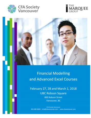
2Advanced Excel Functions and ProceduresThe purpose of this chapter is to review certain Excel functions and procedures usedin the text. These include mathematical, statistical and lookup functions from Excel’sextensive range of functions, as well as much-used procedures such as setting up DataTables and displaying results in XY charts. Also included are methods of summarisingdata sets, conducting regression analyses, and accessing Excel’s Goal Seek and Solver.The objective is to clarify and ensure that this material causes the reader no difficulty.The advanced Excel user may wish to skim the content or use the chapter for furtherreference as and when required. To make the various topics more entertaining and moreinteractive, a workbook AMFEXCEL.xls includes the examples discussed in the text andallows the reader to check his or her proficiency.2.1 ACCESSING FUNCTIONS IN EXCELExcel provides many worksheet functions, which are essentially calculation routines thathave been coded up. They are useful for simplifying calculations performed in the spreadsheet, and also for combining into VBA macros and user-defined functions (topics coveredin Chapters 3 and 4).The Paste Function button (labelled fx) on the standard toolbar gives access to them. (Itwas previously known as the function wizard.) As Figure 2.1 shows, functions are groupedinto different categories: mathematical, statistical, logical, lookup and reference, etc.Figure 2.1 Paste Function dialog box showing the COMBIN function in the Math category

10Advanced Modelling in FinanceHere the Math & Trig function COMBIN has been selected, which produces a briefdescription of the function’s inputs and outputs. For a fuller description, press the Helpbutton (labelled ?).On clicking OK, the Formula palette appears providing slots for entering the appropriateinputs, as in Figure 2.2. The required inputs can be keyed into the slots (as here) or‘selected’ by referencing cells in the spreadsheet (by clicking the buttons to collapse theFormula palette). Note that the palette can be dragged away from its standard position.Clicking the OK button on the palette or the tick on the Edit line enters the formula inthe spreadsheet.Figure 2.2 Building the COMBIN function in the Formula paletteAs well as the Formula palette with inputs for function COMBIN, Figure 2.2 shows theconstruction of the cell formula on the Edit line, with the Paste Function button depressed(in action). Notice also the Paste Name button (labelled Dab) which facilitates pasting ofnamed cells into the formula. (Attaching names to ranges and referencing cell ranges bynames is reviewed in section 2.10.)As well as all Excel functions, the Paste Function button also provides access to theuser-defined category of functions which

2.13.7 Summary of Excel's matrix functions 37 Summary 37 3 Introduction to VBA 39 3.1 Advantages of mastering VBA 39 3.2 Object-oriented aspects of VBA 40 3.3 Starting to write VBA macros 42 3.3.1 Some simple examples of VBA subroutines 42 3.3.2 MsgBox for interaction 43 3.3.3 The writing environment 44 3.3.4 Entering code and executing macros 44