Transcription
7: The CRR Market ModelMarek RutkowskiSchool of Mathematics and StatisticsUniversity of SydneyMATH3075/3975 Financial MathematicsSemester 2, 20167: The CRR Market Model
OutlineWe will examine the following issues:1The Cox-Ross-Rubinstein Market Model2The CRR Call Option Pricing Formula3Call and Put Options of American Style4Dynamic Programming Approach to American Claims5Examples: American Call and Put Options7: The CRR Market Model
PART 1THE COX-ROSS-RUBINSTEIN MARKET MODEL7: The CRR Market Model
IntroductionThe Cox-Ross-Rubinstein market model (CRR model) isan example of a multi-period market model of the stock price.At each point in time, the stock price is assumed to either go‘up’ by a fixed factor u or go ‘down’ by a fixed factor d.Only three parameters are needed to specify the binomialasset pricing model: u d 0 and r 1.Note that we do not postulate that d 1 u.The real-world probability of an ‘up’ mouvement is assumedto be the same 0 p 1 for each period and is assumed tobe independent of all previous stock price mouvements.7: The CRR Market Model
Bernoulli ProcessesDefinition (Bernoulli Process)A process X (Xt )1 t T on a probability space (Ω, F, P) is calledthe Bernoulli process with parameter 0 p 1 if the randomvariables X1 , X2 , . . . , XT are independent and have the followingcommon probability distributionP(Xt 1) 1 P(Xt 0) p.Definition (Bernoulli Counting Process)The Bernoulli counting process N (Nt )0 t T is defined bysetting N0 0 and, for every t 1, . . . , T and ω Ω,Nt (ω) : X1 (ω) X2 (ω) · · · Xt (ω).The process N is a special case of an additive random walk.7: The CRR Market Model
Stock PriceDefinition (Stock Price)The stock price process in the CRR model is defined via an initialvalue S0 0 and, for 1 t T and all ω Ω,St (ω) : S0 u Nt (ω) d t Nt (ω) .The underlying Bernoulli process X governs the ‘up’ and‘down’ mouvements of the stock. The stock price moves upat time t if Xt (ω) 1 and moves down if Xt (ω) 0.The dynamics of the stock price can be seen as an example ofa multiplicative random walk.The Bernoulli counting process N counts the up mouvements.Before and including time t, the stock price moves up Nttimes and down t Nt times.7: The CRR Market Model
Distribution of the Stock PriceFor each t 1, 2, . . . , T , the random variable Nt has thebinomial distribution with parameters p and t.Specifically, for every t 1, . . . , T and k 0, . . . , t we havethat t kP(Nt k) p (1 p)t k .kHence the probability distribution of the stock price St at timet is given by t kk t kP(St S0 u d) p (1 p)t kkfor k 0, 1, . . . , t.7: The CRR Market Model
Stock Price u2d2S0ud. 0.2S0ud2S0d 0.4S0ud3S d20 0.6.S0d3 0.8S0d4 1Figure: Stock Price Lattice in the CRR Model7: The CRR Market Model
Risk-Neutral Probability MeasureProposition (7.1)e onAssume that d 1 r u. Then a probability measure P(Ω, FT ) is a risk-neutral probability measure for the CRR modelM (B, S) with parameters p, u, d, r and time horizon T if andonly if:123X1 , X2 , X3 , . . . , XT are independent under the probabilityemeasure P,e (Xt 1) 1 for all t 1, . . . , T ,0 ep : Pep )d (1 r ),p u (1 ewhere X is the Bernoulli process governing the stock price S.7: The CRR Market Model
Risk-Neutral Probability MeasureProposition (7.2)If d 1 r u then the CRR market model M (B, S) isarbitrage-free and complete.Since the CRR model is complete, the unique arbitrage priceof any European contingent claim can be computed using therisk-neutral valuation formula XFtπt (X ) Bt EPeBTWe will apply this formula to the call option on the stock.7: The CRR Market Model
PART 2THE CRR CALL OPTION PRICING FORMULA7: The CRR Market Model
CRR Call Option Pricing FormulaProposition (7.3)The arbitrage price at time t 0 of the European call optionCT (ST K ) in the binomial market model M (B, S) isgiven by the CRR call pricing formulaT T XXT kKT kT ke (1 ep )T kpC0 S0p̂ (1 p̂) (1 r )Tkkk k̂k k̂whereep 1 r d,u dp̂ epu1 rand k̂ is the smallest integer k such thatk log u d log KS0 d T .7: The CRR Market Model
Proof of Proposition 7.3Proof of Proposition 7.3.The price at time t 0 of the claim X CT (ST K ) can beecomputed using the risk-neutral valuation under PC0 1Ee (CT ) .(1 r )T PIn view of Proposition 7.1, we obtainT X T k1ep (1 ep )T k max 0, S0 u k d T k K .C0 T(1 r )kk 0We note that u kKS0 d T u K log k logdS0 d TS0 u k d T k K 0 d 7: The CRR Market Model
Proof of Proposition 7.3Proof of Proposition 7.3 (Continued).We define k̂ k̂(S0 , T ) as the smallest integer k such that the lastinequality is satisfied. If there are less than k̂ upward mouvementsthere is no chance that the option will expire worthless.Therefore, we obtainC0 T X 1T ke (1 epp )T k S0 u k d T k KT(1 r )kk k̂ T XT kS0ep )T k u k d T kp (1 e(1 r )Tkk k̂T XKT ke (1 e pp )T k(1 r )Tkk k̂7: The CRR Market Model
Proof of Proposition 7.3Proof of Proposition 7.3 (Continued).Consequently,C0 S0 k T kT Xe(1 ep )dTpu1 r1 rkk k̂ T XKT ke (1 epp )T k(1 r )Tkk k̂and thusT T XXT kKT kT ke (1 epp )T kC0 S0p̂ (1 p̂) T(1 r )kkk k̂k k̂where we denote p̂ epu1 r .7: The CRR Market Model
Martingale Approach (MATH3975)Check that 0 p̂ epu1 r 1 whenever 0 ep 1 r du d 1.b be the probability measure obtained by setting p pb inLet PbProposition 7.1. Then the process BS is a martingale under P.For t 0, the price of the call satisfiesbeC0 S0 P(D) KB(0, T ) P(D)where D {ω Ω : ST (ω) K }.Recall thatCt Bt EPe BT 1 (ST K ) Ft Using the abstract Bayes formula, one can show thatb Ft ) KB(t, T ) P(De Ft ).Ct St P(D7: The CRR Market Model
Put-Call ParityIt is possible to derive explicit pricing formula for the calloption at any date t 0, 1, . . . , T .Since CT PT ST K , we see that the following put-callparity holds at any date t 0, 1, . . . , TCt Pt St K (1 r ) (T t) St KB(t, T )whereB(t, T ) (1 r ) (T t)is the price at time t of zero-coupon bond maturing at T .Using Proposition 7.3 and the put-call parity, one can derivean explicit pricing formula for the European put option withthe payoff PT (K ST ) . This is left as an exercise.7: The CRR Market Model
PART 3CALL AND PUT OPTIONS OF AMERICAN STYLE7: The CRR Market Model
American OptionsIn contrast to a contingent claim of a European style, a claimof an American style can by exercised by its holder at anydate before its expiration date T .Definition (American Call and Put Options)An American call (put) option is a contract which gives the holderthe right to buy (sell) an asset at any time t T at strike price K .It the study of an American claim, we are concerned with theprice process and the ‘optimal’ exercise policy by its holder.If the holder of an American option exercises it at τ [0, T ],τ is called the exercise time.7: The CRR Market Model
Stopping TimesAn admissible exercise time should belong to the class ofstopping times.Definition (Stopping Time)A stopping time with respect to a given filtration F is a mapτ : Ω {0, 1, . . . , T } such that for any t 0, 1, . . . , T the event{ω Ω τ (ω) t} belongs to the σ-field Ft .Intuitively, this property means that the decision whetherto stop a given process at time t (for instance, whether toexercise an option at time t or not) depends on the stockprice fluctuations up to time t only.DefinitionLet T [t,T ] be the subclass of stopping times τ with respect to Fsatisfying the inequalities t τ T .7: The CRR Market Model
American Call OptionDefinitionBy an arbitrage price of the American call we mean a priceprocess Cta , t T , such that the extended financial market model– that is, a market with trading in riskless bonds, stocks and anAmerican call option – remains arbitrage-free.Proposition (7.4)The price of an American call option in the CRR arbitrage-freemarket model with r 0 coincides with the arbitrage price of aEuropean call option with the same expiry date and strike price.Proof.It is sufficient to show that the American call option shouldnever be exercised before maturity, since otherwise the issuerof the option would be able to make riskless profit.7: The CRR Market Model
Proof of Proposition 7.4Proof of Proposition 7.4 – Step 1.The argument hinges on the inequality, for t 0, 1, . . . , T ,Ct (St K ) .(1)An intuitive way of deriving (1) is based on no-arbitragearguments.Notice that since the price Ct is always non-negative, itsuffices to consider the case when the current stock price isgreater than the exercise price: St K 0.Suppose, on the contrary, that Ct St K for some t.Then it would be possible, with zero net initial investment, tobuy at time t a call option, short a stock, and invest the sumSt Ct K in the savings account.7: The CRR Market Model
Proof of Proposition 7.4Proof of Proposition 7.4 – Step 1.By holding this portfolio unchanged up to the maturity dateT , we would be able to lock in a riskless profit.Indeed, the value of our portfolio at time T would satisfy(recall that r 0)CT ST (1 r )T t (St Ct ) (ST K ) ST (1 r )T t K 0.We conclude that inequality (1) is necessary for the absenceof arbitrage opportunities.In the next step, we assume that (1) holds.7: The CRR Market Model
Proof of Proposition 7.4Proof of Proposition 7.4 – Step 2.Taking (1) for granted, we may now deduce the propertyCta Ct using simple no-arbitrage arguments.Suppose, on the contrary, that the issuer of an American callis able to sell the option at time 0 at the price C0a C0 .In order to profit from this transaction, the option writerestablishes a dynamic portfolio φ that replicates the valueprocess of the European call and invests the remaining fundsin the savings account.Suppose that the holder of the option decides to exercise it atinstant t before the expiry date T .7: The CRR Market Model
Proof of Proposition 7.4Proof of Proposition 7.4 – Step 2.Then the issuer of the option locks in a riskless profit, sincethe value of his portfolio at time t satisfiesCt (St K ) (1 r )t (C0a C0 ) 0.The above reasoning implies that the European and Americancall options are equivalent from the point of view of arbitragepricing theory.Both options have the same price and an American call shouldnever be exercised by its holder before expiry.Note that the assumption r 0 was necessary to obtain (1).7: The CRR Market Model
American Put OptionRecall that the American put is an option to sell a specifiednumber of shares, which may be exercised at any time beforeor at the expiry date T .For the American put on stock with strike K and expiry dateT , we have the following valuation result.Proposition (7.5)The arbitrage price Pta of an American put option equals Pta max EPe (1 r ) (τ t) (K Sτ ) Ft , t T .τ T [t,T ]For any t T , the stopping time τt which realizes the maximumis given by the expressionτt min {u t Pua (K Su ) }.7: The CRR Market Model
PART 4DYNAMIC PROGRAMMING APPROACHTO AMERICAN CLAIMS7: The CRR Market Model
Dynamic Programming RecursionThe stopping time τt is called the rational exercise timeof an American put option that is assumed to be still aliveat time t.By an application of the classic Bellman principle (1952),one reduces the optimal stopping problem in Proposition 7.5to an explicit recursive procedure for the value process.The following corollary to Proposition 7.5 gives the dynamicprogramming recursion for the value of an American putoption.Note that this is an extension of the backward inductionapproach to the valuation of European contingent claims.7: The CRR Market Model
Dynamic Programming RecursionCorollary (Bellman Principle)Let the non-negative adapted process U be defined recursively bysetting UT (K ST ) and for t T 1noUt max (K St ) , (1 r ) 1 EPe (Ut 1 Ft ) .Then the arbitrage price Pta of the American put option at time tequals Ut and the rational exercise time after time t admits thefollowing representationτt min {u t Uu (K Su ) }.Therefore, τT T and for every t 0, 1, . . . , T 1 1{Ut (K St ) } .τt t1{Ut (K St ) } τt 17: The CRR Market Model
Dynamic Programming RecursionIt is also possible to show directly that the price Pta satisfiesthe recursive relationship, for t T 1,n oaPta max (K St ) , (1 r ) 1 EPe Pt 1 Ftsubject to the terminal condition PTa (K ST ) .In the case of the CRR model, this formula reduces thevaluation problem to the simple single-period case.To show this we shall argue by contradiction. Assume firstthat (2) fails to hold for t T 1. If this is the case, onemay easily construct at time T 1 a portfolio which producesriskless profit at time T . Hence, we conclude that necessarilyn oPTa 1 max (K ST 1 ) , (1 r ) 1 EPe (K ST ) FT .This procedure may be repeated as many times as needed.7: The CRR Market Model
American Put Option: SummaryTo summarise:In the CRR model, the arbitrage pricing of the American putoption reduces to the following recursive recipe, for t T 1,n oadauPta max (K St ) , (1 r ) 1 ep )Pt 1p Pt 1 (1 ewith the terminal conditionPTa (K ST ) .au and P ad represent the values of theThe quantities Pt 1t 1American put in the next step corresponding to the upwardand downward mouvements of the stock price starting from agiven node on the CRR lattice.7: The CRR Market Model
General American ClaimDefinitionAn American contingent claim X a (X , T [0,T ] ) expiring at Tconsists of a sequence of payoffs (Xt )0 t T where the randomvariable Xt is Ft -measurable for t 0, 1, . . . , T and the set T [0,T ]of admissible exercise policies.We interpret Xt as the payoff received by the holder of theclaim X a upon exercising it at time t.The set of admissible exercise policies is restricted to the classT [0,T ] of all stopping times with values in {0, 1, . . . , T }.Let g : R {0, 1, . . . , T } R be an arbitrary function. Wesay that X a is a path-independent American claim with thepayoff function g if the equality Xt g (St , t) holds for everyt 0, 1, . . . , T .7: The CRR Market Model
General American Claim (MATH3975)Proposition (7.6)For every t T , the arbitrage price π(X a ) of an American claimX a in the CRR model equals πt (X a ) max EPe (1 r ) (τ t) Xτ Ft .τ T [t,T ]The price process π(X a ) satisfies the following recurrence relation,for t T 1,n oπt (X a ) max Xt , EPe (1 r ) 1 πt 1 (X a ) Ftwith πT (X a ) XT and the rational exercise time τt equals τt min u t Xu EPe (1 r ) 1 πu 1 (X a ) Fu .7: The CRR Market Model
Path-Independent American Claim: ValuationFor a generic value of the stock price St at time t, we denoteu (X a ) and π d (X a ) the values of the price πaby πt 1t 1 (X )t 1at the nodes corresponding to the upward and downwardmouvements of the stock price during the period [t, t 1],that is, for the values uSt and dSt of the stock price at timet 1, respectively.Proposition (7.7)For a path-independent American claim X a with the payoff processXt g (St , t) we obtain, for every t T 1,n oudπt (X a ) max g (St , t), (1 r ) 1 ep πt 1(X a ) (1 ep ) πt 1(X a ) .7: The CRR Market Model
Path-Independent American Claim: SummaryConsider a path-independent American claim X a with the payofffunction g (St , t). Then:Let Xta πt (X a ) be the arbitrage price at time t of X a .Then the pricing formula becomesn oadauXta max g (St , t), (1 r ) 1 ep ) Xt 1p Xt 1 (1 ewith the terminal condition XTa g (ST , T ). Moreover τt min u t g (Su , u) Xua .The risk-neutral valuation formula given above is valid foran arbitrary path-independent American claim with a payofffunction g in the CRR binomial model.7: The CRR Market Model
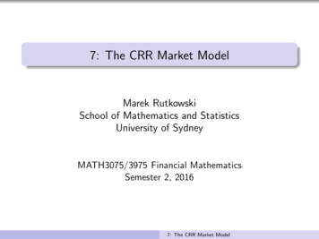
Example: American Call OptionExample (7.1)We consider here the CRR binomial model with the horizondate T 2 and the risk-free rate r 0.2.The stock price S for t 0 and t 1 equalsS0 10,S1u 13.2,S1d 10.8.Let X a be the American call option with maturity date T 2and the following payoff processg (St , t) (St Kt ) .The strike Kt is variable and satisfiesK0 9,K1 9.9,K2 12.7: The CRR Market Model
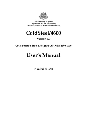
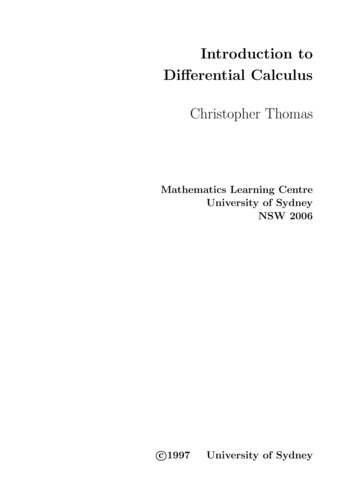
Example: American Call OptionExample (7.1 Continued)We will first compute the arbitrage price πt (X a ) of this optionat times t 0, 1, 2 and the rational exercise time τ0 .Subsequently, we will compute the replicating strategy for X aup to the rational exercise time τ0 .We start by noting that the unique risk-neutral probabilitye satisfiesmeasure Pep 1 r d12 10.8(1 r )S0 S1d 0.5udu d13.2 10.8S1 S1e are given by the firstThe dynamics of the stock price under Pudduexhibit (note that S2 S2 ).The second exhibit represents the price of the call option.7: The CRR Market Model
S uu 17.429ω1 14.256ω2 14.256ω3S2dd 11.664ω42rr80.5 rrrrrrrrS1u 13.2LLLCLLL0.5 LLL L& 0.5 udS2 S0 1077777777770.5777777 S1dduS2r9rr0.5 rrrrrrr 10.8LLLLLL0.5LLLL%7: The CRR Market Model
(17.429 12) 5.4295kkkkkkkkkkkkkkmax (3.3, 3.202) 3.3SSSw;SSSwwSSSwSSSwwwSS)wwww(14.256 12) 2.256wwwwwwwwwwmax (1, 1.7667) 1.7667GGGGGGGGGGGG(14.256 12) 2.256GG5GGkkkkGGkkkkGGkkkG#kkkmax (0.9, 0.94) 0.94SSSSSSSSSSSSSS)(11.664 12) 07: The CRR Market Model
Example: Replicating StrategyExample (7.1 Continued)Holder. The rational holder should exercise the Americanoption at time t 1 if the stock price rises during the firstperiod. Otherwise, the option should be held till time 2.Hence τ0 : Ω {0, 1, 2} equalsτ0 (ω) 1 for ω {ω1 , ω2 }τ0 (ω) 2 for ω {ω3 , ω4 }Issuer. We now take the position of the issuer of the option.At t 0, we need to solve1.2 φ00 13.2 φ10 3.31.2 φ00 10.8 φ10 0.94Hence (φ00 , φ10 ) ( 8.067, 0.983) for all ω.7: The CRR Market Model
Example: Replicating StrategyExample (7.1 Continued)If the stock price rises during the first period, the option isexercised and thus we do not need to compute the strategy attime 1 for ω {ω1 , ω2 }.If the stock price falls during the first period, we solve1.2 φe01 14.256 φ11 2.2561.2 φe01 11.664 φ11 0Hence (φe01 , φ11 ) ( 8.46, 0.8704) for ω {ω3 , ω4 }.Note that φe01 8.46 is the amount of cash borrowed at time1, rather than the number of units of the savings account B.The replicating strategy φ (φ0 , φ1 ) is defined at time 0 forall ω and it is defined at time 1 on the event {ω3 , ω4 } only.7: The CRR Market Model
ll5llllllllllllV1u (φ) 3.3:RRRRRRttRRRtttRRRttRR)tttt tttttttttt(φ00 , φ10 ) ( 8.067, 0.983)HHHHHHHHHHHHHHHHHHHHHH V du (φ) 2.25626llllllllllllle0 , φ1 ) ( 8.46, 0.8704)(φ11RRRRRRRRRRRRR(V2dd (φ) 07: The CRR Market Model
PART 5IMPLEMENTATION OF THE CRR MODEL7: The CRR Market Model
Derivation of u and d from r and σWe fix maturity T and we assume that the continuouslycompounded interest rate r is such that B(0, T ) e rT .From the market data for stock prices, one can estimate thestock price volatility σ per one time unit (typically, one year).Note that until now we assumed that t 0, 1, 2, . . . , T , whichmeans that t 1. In general, the length of each period canbe any positive number smaller than 1. We set n T / t.Two widely used conventions for obtaining u and d from σand r are:The Cox-Ross-Rubinstein (CRR) parametrisation:u eσ tand d 1.uThe Jarrow-Rudd (JR) parameterisation:u e 2r σ2 t σ tandd e 2r σ2 t σ t7: The CRR Market Model.
The CRR parameterisationProposition (7.8)Assume that Bk t (1 r t)k for every k 0, 1, . . . , n andu d1 e σ t in the CRR model. Then the risk-neutrale satisfiesprobability measure P2 1 r σ2 e t o( t)P (St t St u St ) 22σprovided that t is sufficiently small.Proof of Proposition 7.8.The risk-neutral probability measure for the CRR model is given bye (St t St u St ) ep P1 r t du d7: The CRR Market Model
The CRR parameterisationProof of Proposition 7.8.Under the CRR parametrisation, we obtain 1 r t d1 r t e σ t ep .u de σ t e σ tThe Taylor expansions up to the second order term areeσe σ t t σ2 1 σ t t o( t)2 σ2 1 σ t t o( t)27: The CRR Market Model
The CRR parameterisationProof of Proposition 7.8.By substituting the Taylor expansions into the risk-neutralprobability measure, we obtainep 21 r t 1 σ t σ2 t o( t) 221 σ t σ2 t 1 σ t σ2 t o( t) 2σ t r σ2 t o( t) 2σ t o( t)2 1 r σ2 t o( t) 22σas was required to show.7: The CRR Market Model
The CRR parameterisationTo summarise, for t sufficiently small, we getep 1 r t e σeσ t e σ t t21 r σ2 t. 22σNote that 1 r t e r t when t is sufficiently small.Hence the risk-neutral probability measure can also berepresented as followsep eσ t t .e σ te r t e σMore formally, if we define r̂ such that (1 r̂ )n e rT for afixed T and n T / t then r̂ r t since ln(1 r̂) r tand ln(1 r̂) r̂ when r̂ is close to zero.7: The CRR Market Model
Example: American Put OptionExample (7.2 – CRR Parameterisation)Let the annualized variance of logarithmic returns be σ 2 0.1.The interest rate is set to r 0.1 per annum.Suppose that the current stock price is S0 50.We examine European and American put options with strikeprice K 53 and maturity T 4 months (i.e. T 31 ).The length of each period is t Hence n T t112 ,that is, one month. 4 steps.We adopt the CRR parameterisation to derive the stock price.Then u 1.0956 and d 1/u 0.9128.We compute 1 r t 1.00833 e r t and ep 0.5228.7: The CRR Market Model
Example: American Put OptionExample (7.2 Continued)Stock Price Process7572.03647065.75166560.0152Stock .533.544.5t/ tFigure: Stock Price Process7: The CRR Market Model
Example: American Put OptionExample (7.2 Continued)Price Process of the European Put Option750700650.67199Stock 3.544.5t/ tFigure: European Put Option Price7: The CRR Market Model
Example: American Put OptionExample (7.2 Continued)Price Process of the American Put Option750700650.67199Stock .544.5t/ tFigure: American Put Option Price7: The CRR Market Model
Example: American Put OptionExample (7.2 Continued)1: Exercise the American Put; 0: Hold the American Option801701Stock Price10600050100101140113000.511.522.533.544.5t/ tFigure: Rational Exercise Policy7: The CRR Market Model
The JR parameterisationThe next result deals with the Jarrow-Rudd parametrisation.Proposition (7.9)Let Bk t (1 r t)k for k 0, 1, . . . , n. We assume thatu eandd e 2r σ22r σ2 t σ t t σ t.e satisfiesThen the risk-neutral probability measure Pe (St t St u St ) 1 o( t)P2provided that t is sufficiently small.7: The CRR Market Model
The JR parameterisationProof of Proposition 7.9.Under the JR parametrisation, we have1 r t de p u de 1 r t e2r σ2 t σ t2r σ2 e t σ t2r σ2 . t σ tThe Taylor expansions up to the second order term areee2 t σ t2 t σ t r σ2 r σ2and thusep 1 r t σ t o( t) 1 r t σ t o( t)1 o( t).27: The CRR Market Model
Example: American Put OptionExample (7.3 – JR Parameterisation)We consider the same problem as in Example 7.2, but withparameters u and d computed using the JR parameterisation.We obtain u 1.1002 and d 0.9166.As before, 1 r t 1.00833 e r t , but ep 0.5.We compute the price processes for the stock, the Europeanput option, the American put option and we find the rationalexercise time.When we compare with Example 7.2, we see that the resultsare slightly different than before, although it appears that therational exercise policy is the same.The CRR and JR parameterisations are both set to approachthe Black-Scholes model.For t sufficiently small, the prices computed under the twoparametrisations will be very close to one another.7: The CRR Market Model
Example: American Put OptionExample (7.3 Continued)Stock Price Process8073.24717066.5787Stock 0.511.522.533.544.5t/ tFigure: Stock Price Process7: The CRR Market Model
Example: American Put OptionExample (7.3 Continued)Price Process of the European Put Option800700Stock 2.533.544.5t/ tFigure: European Put Option Price7: The CRR Market Model
Example: American Put OptionExample (7.3 Continued)Price Process of the American Put Option800700Stock 2.533.544.5t/ tFigure: American Put Option Price7: The CRR Market Model
Example: American Put OptionExample (7.3 Continued)1: Exercise the American Put; 0: Hold the American Option801701Stock Price10600050100101140113000.511.522.533.544.5t/ tFigure: Rational Exercise Policy7: The CRR Market Model
The stock price moves up at time t if X t(ω) 1 and moves down if X t(ω) 0. The dynamics of the stock price can be seen as an example of a multiplicative random walk. The Bernoulli counting process N counts the up mouvements. Before and including time t, the stock price moves up N t times and down t N t times. 7: The CRR Market Model