Transcription
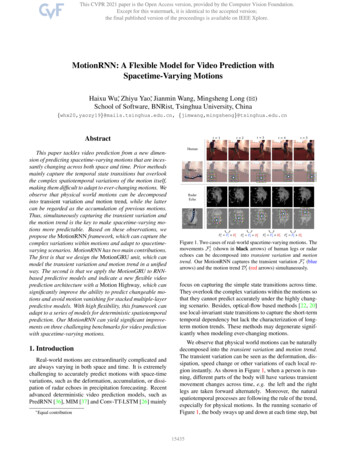
MotionRNN: A Flexible Model for Video Prediction withSpacetime-Varying MotionsHaixu Wu*, Zhiyu Yao*, Jianmin Wang, Mingsheng Long (B)School of Software, BNRist, Tsinghua University, China{whx20,yaozy19}@mails.tsinghua.edu.cn, {jimwang,mingsheng}@tsinghua.edu.cnAbstract𝑡 1𝑡 2𝑡 3𝑡 4𝑡 5HumanThis paper tackles video prediction from a new dimension of predicting spacetime-varying motions that are incessantly changing across both space and time. Prior methodsmainly capture the temporal state transitions but overlookthe complex spatiotemporal variations of the motion itself,making them difficult to adapt to ever-changing motions. Weobserve that physical world motions can be decomposedinto transient variation and motion trend, while the lattercan be regarded as the accumulation of previous motions.Thus, simultaneously capturing the transient variation andthe motion trend is the key to make spacetime-varying motions more predictable. Based on these observations, wepropose the MotionRNN framework, which can capture thecomplex variations within motions and adapt to spacetimevarying scenarios. MotionRNN has two main contributions.The first is that we design the MotionGRU unit, which canmodel the transient variation and motion trend in a unifiedway. The second is that we apply the MotionGRU to RNNbased predictive models and indicate a new flexible videoprediction architecture with a Motion Highway, which cansignificantly improve the ability to predict changeable motions and avoid motion vanishing for stacked multiple-layerpredictive models. With high flexibility, this framework canadapt to a series of models for deterministic spatiotemporalprediction. Our MotionRNN can yield significant improvements on three challenging benchmarks for video predictionwith spacetime-varying motions.1. IntroductionReal-world motions are extraordinarily complicated andare always varying in both space and time. It is extremelychallenging to accurately predict motions with space-timevariations, such as the deformation, accumulation, or dissipation of radar echoes in precipitation forecasting. Recentadvanced deterministic video prediction models, such asPredRNN [36], MIM [37] and Conv-TT-LSTM [26] mainly* EqualcontributionMotionRadarEchoMotion𝐹%" 𝐹%# 𝐷%"𝐹!" 𝐹!# 𝐷!"𝐹 " 𝐹 # 𝐷 "𝐹&" 𝐹&# 𝐷&"Figure 1. Two cases of real-world spacetime-varying motions. Themovements Ftl (shown in black arrows) of human legs or radarechoes can be decomposed into transient variation and motiontrend. Our MotionRNN captures the transient variation Ft′ (bluearrows) and the motion trend Dtl (red arrows) simultaneously.focus on capturing the simple state transitions across time.They overlook the complex variations within the motions sothat they cannot predict accurately under the highly changing scenario. Besides, optical-flow based methods [22, 20]use local-invariant state transitions to capture the short-termtemporal dependency but lack the characterization of longterm motion trends. These methods may degenerate significantly when modeling ever-changing motions.We observe that physical world motions can be naturallydecomposed into the transient variation and motion trend.The transient variation can be seen as the deformation, dissipation, speed change or other variations of each local region instantly. As shown in Figure 1, when a person is running, different parts of the body will have various transientmovement changes across time, e.g. the left and the rightlegs are taken forward alternately. Moreover, the naturalspatiotemporal processes are following the rule of the trend,especially for physical motions. In the running scenario ofFigure 1, the body sways up and down at each time step, but15435
the man keeps moving forward from left to right followingthe unchanging tendency. The motion follows the characteristics behind the physical world in a video sequence, suchas inertia for objects, meteorology for radar echoes, or otherphysical laws, which can be seen as the motion trend of thevideo. Considering the decomposition of the motion, weshould capture the transient variation and the motion trendfor better space-time varying motion prediction.We go beyond the previous state-of-the-art methods fordeterministic spatiotemporal prediction [36, 37, 26] andpropose a novel MotionRNN framework. To enable moreexpressive modeling of the spacetime-varying motions, MotionRNN adapts a MotionGRU unit for high-dimensionalhidden-state transitions, which is specifically designed tocapture the transient variation and the motion trend respectively. Inspired by the residual shortcuts in the ResNet [10],we improve the Motion Highway across layers within ourframework to prevent the captured motions from vanishingand provide useful contextual spatiotemporal informationfor the MotionRNN. Our MotionRNN is flexible and can beeasily adapted to the existing predictive models. Besides,MotionRNN achieves new state-of-the-art performance onthree challenging benchmarks: a real-world human motionbenchmark, a precipitation nowcasting benchmark, and asynthetic varied flying digits benchmark. The contributionsof this paper are summarized as follows: Based on the key observation that the motion canbe decomposed to transient variation and the motiontrend, we design a new MotionGRU unit, which couldcapture the transient variation based on the spatiotemporal information and obtain the motion trend from theprevious accumulation in a unified way. We propose the MotionRNN framework, which unifiesthe MotionGRU and a new Motion Highway structureto make spacetime-varying motions more predictableand to mitigate the problem of motion vanishing acrosslayers in the existing predictive models. Our MotionRNN achieves the new state-of-the-art performance on three challenging benchmarks. And it isflexible to be applied together with a rich family ofpredictive models to yield consistent improvements.2. Related Work2.1. Deterministic Video PredictionRecurrent neural networks (RNNs) have been wildlyused in the field of video prediction to model the temporal dependencies in the video [19, 17, 24, 7, 6, 15, 22, 12,32, 20, 9, 38, 26]. To learn spatial and temporal content anddynamics in a unified network structure, Shi et al. [21] proposed the convolutional LSTM (ConvLSTM), extending theLSTM with convolutions to maintain spatial informationin the sequence model. The fusion of CNNs and LSTMsmakes the predictive models capable to capture the spatiotemporal information. Finn et al. extended ConvLSTMfor robotics to predict the transformation kernel weights between robot states. Wang et al. [36] introduced PredRNN,which makes the memory state update along a zigzag statetransition path across stacked recurrent layers using the STLSTM cell. For capturing long-term dynamics, E3D-LSTM[35] incorporated 3D convolution and memory attentioninto the ST-LSTM, which can capture the long-term videodynamics. Su et al. [26] presented a high-order convolutionLSTM (Conv-TT-LSTM) to learn the spatiotemporal correlations by combining the history convolutional features.Still, previous spatiotemporal predictive models mainlyfocus on spatiotemporal state transitions but ignore internal motion variations. When it comes to instantly-changingmotions, these predictive models may not behave well. Tolearn the coherence between frames, some video predictionmethods are based on the optical flow [27, 23]. SDC-Net[20] learns the transformation kernel and kernel offsets between frames based on the optical flow. TrajGRU [22] alsofollows the idea of optical flow to learn the receptive areaoffsets for a special application of precipitation nowcasting.Villegas et al. [31] leveraged the optical flow for short-termdynamic modeling. These optical-flow based methods capture the short-term temporal dynamics effectively. However, they only treat the video as the instantaneous translation of pixels between adjacent frames and may ignore themotion trend of object variations.Note that these methods are generally based on the RNN,such as LSTMs. In this paper, we propose a flexible externalmodule for RNN-based predictive models without changingtheir original predictive framework. Unlike previous predictive learning methods, our approach focuses on modelingthe within-motion variations, which could learn the explicittransient variation and remember the motion trend in a unified way. Our method naturally complements existing methods for learning spatiotemporal state transitions and can beapplied with them for more powerful video prediction.2.2. Stochastic Video PredictionIn addition to these deterministic video prediction models, some recent literature has explored the spatiotemporal prediction problem by modeling the future uncertainty.These models are based on adversarial training [16, 33, 28]or variational autoencoders (VAEs) [1, 28, 7, 14, 30, 4, 8].These stochastic models could partially capture the spatiotemporal uncertainty by estimating the latent distributionfor each time step. They did not attempt to explicitly modelthe motion variation, which is different from our MotionRNN. Again, MotionRNN can be readily applied with thesestochastic models by replacing their underlying backbones.15436
3. MethodsRecall our observation as shown in Figure 1: real-worldmotions can be decomposed into the transient variation andmotion trend. In the spirit of this observation, we proposethe flexible MotionRNN framework with a motion highway,which could effectively enhance the ability to adapt to thespacetime-varying motions and avoid the motion vanishing.Further, we propose a specifically designed unit named MotionGRU, which can capture the transient variation and motion trend in a unified recurrent cell. This section will firstdescribe the MotionRNN architecture and illustrate how toadapt MotionRNN to the existing RNN-based predictivemodels. Next, we will present the unified modeling of transient variation and motion trend in the MotionGRU unit.3.1. MotionRNNTypically, RNN-based spatiotemporal predictive models are in the forms of stacked blocks, as shown in Figure 2. Here we use each block to indicate the predictiveRNN unit, such as ConvLSTM [21] or ST-LSTM [36]. Inthis framework, the hidden states transit between predictiveblocks and are controlled by the inner recurrent gates. However, when it comes to spacetime-varying motions, the gatecontrolled information flow would be overwhelmed by incessantly making quick responses to the transient variationsof motions. Besides, it also lacks motion trend modeling.H t3HBlock3t3H t 1BlockC 3tH2tBlockH1tC1tBlockBlockBlock2t 1BlockBlockX lt2Ht 1BlockBlock1H t 11t 1F lt-1D lt-12Ct 1C 2tH t1HMotionHighway3Ct 1HH 2t.3t 11t 1CD ltH tlHBlockF ltMotionGRUBlockBlockltHIn detail, the MotionRNN framework inserts the MotionGRU between layers of the original RNN blocks. Take ConvLSTM [21] as an example. After the first layer, the overallequations for the l-th layer at time step t are as follows:llXtl , Ftl , Dtl MotionGRU(Htl , Ft 1, Dt 1)l 1l 1Htl 1 , Ctl 1 Block(Xtl , Ht 1, Ct 1)Htl 1 Htl 1 (1 ot ) (1)Htl ,where l {1, 2, · · · , L}. Tensors Ftl and Dtl denote thetransient filter and the trending momentum from MotionGRU respectively. We will give detailed descriptions to MotionGRU in the next section. The input Xtl of the Block hasl 1l 1been transited by MotionGRU. Ht 1, Ct 1are the hiddenstate and memory state from the previous time step respectively, which are the same as original predictive blocks. otis the output gate of the RNN-based predictive block, whichreveals the constantly updated memory in LSTMs.The last equation presents the motion highway, whichcompensates the predictive block’s output by the previoushidden state Htl . We reuse the output gate to expose the desired unchanging content information. This highway connection provides extra details to the hidden states and balances the invariant part and the changeable motion part.Note that MotionRNN does not change the state transition flows in the original predictive models. Thus, with thishigh flexibility, MotionRNN can adapt to a rich family ofpredictive frameworks, such as ConvLSTM [21], PredRNN[36], MIM [37], E3D-LSTM [35], and other RNN-basedpredictive models. It can significantly enhance spacetimevarying motion modeling of the existing predictive models.3.2. MotionGRUBlock.Figure 2. An overview of typical architecture of predictive frameworks: RNN-based spatiotemporal predictive networks (left), MotionRNN framework (right) which embeds the MotionGRU (bluecircles) between layers of the original models. The blue dashedlines between stacked layers present the Motion Highway.To tackle the challenge of spacetime-varying motionsmodeling, the MotionRNN framework incorporates the MotionGRU unit between the stacked layers as an operatorwithout changing the original state transition flow (Figure2). MotionGRU can capture the motion and conduct a statetransition to the hidden states based on the learned motion.However, we find that motion will blur and even vanishwhen the transited features pass through multi-layers. Motivated by this observation, MotionRNN introduces the Motion Highway to provide an alternative quick route for themotion context information. We find that Motion Highwaycould effectively avoid motion blur and constrain the objectin the right location from the visualization in Figure 6.As mentioned above, towards modeling the spacetimevarying motions, our approach presents the MotionGRUunit to conduct motion-based state transitions by modelingthe motion variation. In video prediction, the motion can bepresented as pixels displacement corresponding to the hidden states transitions in RNNs. We use the MotionGRU tolearn the pixel offsets between adjacent states. The learnedpixel-wise offsets are denoted by motion filter Ftl . Considering that real-world motions are the composition of transient variations and motion trends, we specifically designtwo modules in the MotionGRU to model these two components respectively (Equation 4).3.2.1Transient VariationIn a video, the transient variation at each time step is notonly based on the spatial context but also presents high temporal coherence. For example, the waving hands of a manfollow a nearly continuous arm rotation angle between adjacent frames. Motivated by the spatiotemporal coherence of15437
XltDecgtFltwarpFltF‘t 𝑋!"#D ltTransientVariation D lt 𝑋!%#𝑋! TrendingMomentum 𝐹!"# 𝐹!%#𝐹! WarpWarpWarp ut1-rtEncmomentumXSdate 𝐻! 𝐻!"#HltlF t-1lD t-1Video TimeFigure 3. MotionGRU unit’s architecture. The blue part is to capture the transient variation Ft′ . The trending momentum Dtl accumulates the motion tendency in an accumulation way (red part).transient variations, we adapt a ConvGRU [22] to learn thetransient variation. With this recurrent convolutional network, the learned transient variation could consider the instant states and maintain the spatiotemporal coherence ofvariations. The equations of the transient-variation learnerof the l-th MotionGRU at time step t are shown as follows:ut rt zt l])σ Wu Concat([Enc(Htl ), Ft 1 llσ Wr Concat([Enc(Ht ), Ft 1 ])tanh Wz Concat([Enc(Htl ), rt lFt 1]) (2)lFt′ ut zt (1 ut ) Ft 1. lWe use Ft′ Transient Ft 1, Enc(Htl ) to summarize theabove equations. σ is the sigmoid function, Wu , Wr andWz denotes the 1 1 convolution kernel, and denotethe convolution operator and the Hadamard product respectively. ut and rt are the update gate and reset gate in ConvGRU [22], and zt is the reseted feature of current moment.Enc(Htl ) encodes the input from the last predictive block.lFt 1presents motion filter from the previous time step forcapturing the transient variations. Transient variation Ft′ forcurrent frame is calculated with the update gate ut . Notethat transient variation Ftl presents the transition of eachpixel’s position between adjacent states. Thus, all the gates,zt , and Ftl are in the offset space, which are learned filtersand different from spatiotemporal states Htl , Ctl .3.2.2 𝐻!%#Figure 4. State transitions by MotionGRU. The motion filter Ftlis combined by the transient variation (blue square) and trendingmomentum (red square). The new transited state is obtained bythe Warp operation based on the learned motion filter.pattern of motion variation. We use the previous motion fillter Ft 1as the estimation of the current motion trend andget the momentum update function as follows: lll(3) α Ft 1 Dt 1,Dtl Dt 1where α is the step size of momentum update and Dtl is thelearned trending momentum. We denote the above equall. With momentum uption as Dtl Trend Ft 1, Dt 1ldate, Dt convergences to the weighted sum of motion filtersFtl , which can be viewed as the motion trend in the pastlpresentsperiod. In the running example (Figure 4), Ft 1lthe motion of the last moment and Dt denotes the forwardtrend learned from the past. By momentum updating, thistendency estimation is of larger coefficient over time. Notethat the trending momentum Dtl is the momentum updateof motion filter Ftl and is also in the offset space, whichpresents the learned motion trend of pixels in a video.3.2.3By implementing the key observation of motion decomposition, we design MotionGRU as the following procedure: lFt′ Transient Ft 1, Enc(Htl ) llDtl Trend Ft 1, Dt 1Ftl Ft′ Dtlmlt Broadcast σ(Whm Enc(Htl )) Ht′ mlt Warp Enc(Htl ), FtlTrending MomentumIn the running scenario, the man’s body sways up and downat each step while the man keeps moving forward. In thiscase, the motion is following a forward trend. In video prediction, we usually have to go through the whole frame sequence to get the motion trend. However, the future is unreachable. This dilemma is similar to reward prediction inreinforcement learning. Inspired by Temporal Differencelearning [27], we use an accumulating way to capture theOverall Procedure for MotionGRU gt σ W1 1 Concat([Dec(Ht′ ), Htl ])(4) lXtl gt Ht 1 (1 gt ) Dec(Ht′ ),where t denotes the time step and l {1, · · · , L} denotes the current layer, Transient(·) and Trend(·) presentthe transient-variation learner and trending-momentum updater respectively. Ft′ and Dtl denote the transient variationand trending momentum of the current frame. Based on the15438
observation of motion decomposition, the motion filter Ftlis the combination of transient variation and trending momentum. mlt is the mask for motion filter and Broadcast(·)means the broadcast operation with kernel Whm to keep tensor dimension consistent to Ht′ .For the state transition, we use the warp operation [2, 3]to map the pixels from the previous state to the position inthe next state, which is widely used in different fields ofvideo analysis, such as video style transfer [5] and videorestoration [34]. Here Warp(·) denotes the warp operationwith bilinear interpolation. As shown in Figure 4, warping the previous state by the learned motion Ftl , we canexplicitly incorporate motion variation into the transition ofhidden states. More details about the warp operation in MotionGRU can be found in the supplementary materials. Asshown in Figure 3, the final output Xtl of MotionGRU is agate gt controlled result from the input Htl and the decoderoutput, in which the decoder output has been explicitly transited by warp operation based on the motion filter Ftl .Overall, by capturing the transient variation and motiontrend separately and fusing them in a unified unit, MotionGRU can effectively model the spacetime-varying motions.With MotionGRU and Motion Highway, our MotionRNNframework can be applied to scenarios with ever-changingmotions, which seamlessly compensates existing models.4. ExperimentsWe extensively evaluate our proposed MotionRNN onthe following three challenging benchmarks.Human motions.This benchmark is built on the Human3.6M [11] dataset, which contains human actions fromreal world of 17 different scenarios with 3.6 million poses.We resize each RGB frame to the resolution of 128 128.Real-world human motion is much more complicated. Forexample, when a person is walking, different parts of thehuman body will have diverse transient variations, e.g. thearms and legs are bending, the body is swaying. The complex motion variations will make the prediction of real human motion a really challenging task.Precipitation nowcasting.Precipitation nowcasting isa vital application of video prediction. It is challenging topredict the accumulation, deformation, dissipation, or diffusion of radar echos reflecting severe weather. This benchmark uses the Shanghai radar dataset, which contains evolving radar maps from Shanghai weather bureau. The Shanghai dataset has 40, 000 consecutive radar observations, collected every 12 minutes, with 36, 000 sequences for trainingand 4, 000 for testing. Each frame is resized to the resolution of 64 64.Varied moving digits.We introduce the Varied Moving MNIST (V-MNIST) dataset consisting of sequences offrames with a resolution of 64 64. Previous MovingMNIST [25] or Moving MNIST [22] digits move witha lower velocity without digits variations. By contrast, ourvaried Moving MNIST forces all digits to move, rotate, andscale simultaneously. The V-MNIST are generated on thefly by sampling two different MNIST digits, with 100, 000sequences for training and 10, 000 for testing.Backbone models. To verify the universality of MotionRNN, we use the following predictive models as our backbone models including ConvLSTM [21], PredRNN [36],MIM [37] and E3D-LSTM [35]. On all benchmarks, ourMotionRNN based on these models has four stacked blockswith 64-channel hidden states. For E3D-LSTM, we replacethe encoder and decoder inside the MotionGRU with 3Dconvolutions to downsample the 3D feature map to 2D andkeep the other operations unchanged.Implementation details. Our method is trained with theL1 L2 loss [35] to enhance the sharpness and smoothnessof the generated frames simultaneously, using the ADAM[13] optimizer with an initial learning rate of 3 10 4 . Themomentum factor α is set to 0.5. For memory efficiency,the learned filter size of MotionGRU is set to 3 3. Thebatch size is set to 8, and the training process is stopped after 100, 000 iterations. All experiments are implemented inPyTorch [18] and conducted on NVIDIA TITAN-V GPUs.4.1. Human MotionSetups. We follow the experimental setting in MIM [37],which uses the previous 4 frames to generate the future4 frames. As for evaluation metrics, we use the framewise structural similarity index measure (SSIM), the meansquare error (MSE), the mean absolute error (MAE) to evaluate our models. Besides these common metrics, we alsouse the Fréchet Video Distance (FVD) [29], which is a metric for qualitative human judgment of generated videos. TheFVD could measure both the temporal coherence of thevideo content and the quality of each frame.Results. As shown in Table 1, our proposed MotionRNNpromotes diverse backbone predictive models with consistent improvement in quantitative results. Significantly, withMotionRNN the performance improves 29% in MSE and22% in MAE using the PredRNN as the backbone. Our approach also promotes the FVD, which means the predictionperforms better in motion consistency and frame quality. Toour best knowledge, MotionRNN based on PredRNN hasachieved the state-of-the-art performance on Human3.6M.As for qualitative results, we show a case of walking in Figure 5. In this case, the human has a left movement tendencywith transient variations across different body parts. Theframes generated by MotionRNN are richer in detail andless blurry than those of other models, especially for the15439
Table 1. Quantitative results of Human3.6M upon different network backbones ConvLSTM [21], MIM [37], PredRNN [36] andE3D-LSTM [35]. A lower MSE, MAE or FVD, or a higher SSIMindicates a better prediction.MethodSSIM MSE/10 MAE/100 FVDTrajGRU [22]0.80142.218.626.9Conv-TT-LSTM [26] 0.79147.418.926.2ConvLSTM [21]0.77650.418.928.4 MotionRNN0.80044.318.626.9MIM [37]0.79042.917.821.8 MotionRNN0.84135.114.918.3PredRNN [36]0.78148.418.924.7 MotionRNN0.84634.214.817.6E3D-LSTM [35]0.86949.416.623.7 MotionRNN0.88144.515.821.7Ground Truth & PredictionsInputs𝑡 4𝑡 5𝑡 6𝑡 7𝑡 8 ConvLSTMTrajGRUTable 2. Parameters and computations comparison of MotionRNNusing diverse backbone models. FLOPs denotes the number ofmultiplication operations for a human sequence prediction, whichpredicts the future 4 frames based on the previous 4 frames.MethodConvLSTM MotionRNNPredRNN MotionRNNMIM MotionRNNE3D-LSTM MotionRNNParams(MB)4.415.21( 18%)6.417.01( 9.3%)9.7910.4( 6.2%)20.421.3( 4.4%)FLOPs(G)31.636.6( 16%)46.049.5( 7.6%)70.273.7( 5.0%)292303( 3.8%)MSE 12%29%18%10%Table 3. The ablation of MotionRNN with respect to Motion Highway (MH), Transient Variation (TV) and Trending Momentum(TM) on the Human3.6M dataset. denotes the MSE improvements over PredRNN.MethodMHPredRNN Motion Highway MotionGRU w/o Momentum MotionGRU w/o Transient MotionGRU MotionRNN w/o Momentum MotionRNN w/o Transient MotionRNNTV TM MSE1048.442.541.543.540.338.940.634.2 12%14%10%17%20%16%29%MIME3D-LSTMPredRNNPredRNN MotionRNNtions, as shown in Table 2. MotionRNN improves the performance of the PredRNN significantly (MSE: 48.4 34.2,SSIM: 0.781 0.846) with only 9.3% additional parameters and 7.6% increased computations. The increase of themodel size is the same among different predictive frameworks because MotionRNN is only used as an external operator for hidden states across layers. The growth of thecomputations is also controllable. Based on these observations, we can see that our MotionRNN is a flexible model,which can improve the performance significantly on spatiotemporal variation modeling without significant sacrificein model size or computation cost.Figure 5. Prediction frames on the human motion benchmark.arms and legs. PredRNN and MIM may present the prediction in good sharpness but fail to bend the left elbow, andthe predicted legs are also blurry. By contrast, MotionRNNcould predict the sharpest sequence compared with previous methods and largely enrich the detail for each part ofthe body, especially for the arms and legs. What’s more, thepose prediction for the arms and the legs is also predictedmore precisely, which means our approach could not onlymaintain the details but perform well in motion capturing.Parameters and computations analysis. We measurethe complexity in terms of both model size and computa-Ablation study. As shown in Table 3, we analyze theeffectiveness of each part from our MotionRNN. Onlyby adopting the Motion Highway we could get a fairlygood promotion (12% ) indicating the Motion Highwaycan maintain the information of the motion context andcompensate existing models for the additional useful information. Only adopting the MotionGRU without MotionHighway makes the MotionRNN achieve 17% improvement. From the quantitative results described in Table 3,we could easily find that the Motion Highway and MotionGRU can promote each other and achieve better improvement (29% ). Furthermore, from the qualitative results15440
shown in Figure 6, we can find without the Motion Highway, the predictions lose details of the arms and have thepositional skewing. Thus we can verify the effect of ourMotion Highway, which can compensate necessary content details to the MotionGRU and constrained the motion in the right area. More visualization can be found insupplementary materials. Besides, the learned trending momentum and transient variation give 9% and 13% extra promotions respectively, indicating that both parts of motiondecomposition are effective for video prediction.GroundTruth! 5! 6! 7! 8Table 4. Quantitative results of the Shanghai dataset upon differentnetwork backbone. A lower GDL or a higher CSI means a betterprediction performance.MethodTrajGRUConv-TT-LSTMConvLSTM MotionRNNMIM MotionRNNPredRNN MotionRNNE3D-LSTM .79.67InputsPredRNN MotionRNN! 1! 5! 6! 7! 8! 5! 6! 7! 8! 10.6230.5900.621Ground Truth & Predictions! 5! 7! 9! 11! 13! 15PredRNN MotionRNN-Motion HighwayPredRNNFigure 6. The qualitative case for the ablation study of the MotionHighway, using the red box to box out of the body.PredRNN MotionRNNPredRNNPredRNN MotionRNNFigure 8. Prediction examples on the Shanghai radar echo dataset.Figure 7. The sensitivity analysis of hyper-parameter α.Hyper-parameters. We show the sensitivity analysis ofthe training hyper-parameter α for trending momentum inFigure 7. Our MotionRNN based on PredRNN and ConvLSTM achieves great performance when α 0.5 and isrobust and easy to tune in the range of 0.5 to 0.7. We havesimilar results on the other two benchmarks and thus set αto 0.5 throughout the experiments.4.2. Precipitation NowcastingSetups.We forecast the next 10 radar echo framesfrom the previous 5 observations, covering weather conditions in the next two hours. We use the gradient difference loss (GDL) [16] to measure the sharpness of theprediction frames. A lower GDL indicates a higher sharpness similarity of ground truth. Further, for radar echointensities, we convert the pixel values in dBZ and compare the Critical Success Index (CSI) with 30 dBZ, 40dBZ, 50 dBZ as thresholds, respectively. CSI is defined asHitsCSI Hits Misses FalseAlarms, where hits correspond to thetrue positive, misses correspond to the false positive, andfalse alarms correspond to the false negative. A higher CSIindicates better forecasting performance. Compared withMSE, the CSI metric is particularly sensitive to the highintensity echoes, always with high changeable motions.Results. We provide quantitative results in Table 4, ourMotionRNN using the state-of-the-art model E3
adapt MotionRNN to the existing RNN-based predictive models. Next, we will present the unified modeling of tran-sient variation and motion trend in the MotionGRU unit. 3.1. MotionRNN Typically, RNN-based spatiotemporal predictive mod-els are in the forms of stacked blocks, as shown in Fig-ure 2. Here we use each block to indicate the predictive