Transcription
Linear Algebra & GeometryRoman Schubert1May 22, 20121School of Mathematics, University of Bristol.c University of Bristol 2011 This material is copyright of the University unless explicitly stated otherwise. It is provided exclusively for educational purposes at the University and is to be downloadedor copied for your private study only.
2These are Lecture Notes for the 1st year Linear Algebra and Geometry course in Bristol.This is an evolving version of them, and it is very likely that they still contain many misprints.Please report serious errors you find to me (roman.schubert@bristol.ac.uk) and I will postan update on the Blackboard page of the course.These notes cover the main material we will develop in the course, and they are meantto be used parallel to the lectures. The lectures will follow roughly the content of the notes,but sometimes in a different order and sometimes containing additional material. On theother hand, we sometimes refer in the lectures to additional material which is covered inthe notes. Besides the lectures and the lecture notes, the homework on the problem sheetsis the third main ingredient in the course. Solving problems is the most efficient way oflearning mathematics, and experience shows that students who regularly hand in homeworkdo reasonably well in the exams.These lecture notes do not replace a proper textbook in Linear Algebra. Since LinearAlgebra appears in almost every area in Mathematics a slightly more advanced textbookwhich complements the lecture notes will be a good companion throughout your mathematicscourses. There is a wide choice of books in the library you can consult.11c University of Bristol 2013 This material is copyright of the University unless explicitly stated otherwise.It is provided exclusively for educational purposes at the University and is to be downloaded or copied for yourprivate study only.
Contents1 The1.11.21.3Euclidean plane and complexThe Euclidean plane R2 . . . . .The dot product and angles . . .Complex Numbers . . . . . . . .numbers. . . . . . . . . . . . . . . . . . . . . . . . . . . . . . . . . . . . . . . . . . . . . . . . . . . . . . . . . . . . . . . . . . . . . . . . .559102 Euclidean space Rn2.1 Dot product . . . . . . . . . . . . . . . . . . . . . . . . . . . . . . . . . . . . .2.2 Angle between vectors in Rn . . . . . . . . . . . . . . . . . . . . . . . . . . .2.3 Linear subspaces . . . . . . . . . . . . . . . . . . . . . . . . . . . . . . . . . .151719203 Linear equations and Matrices3.1 Matrices . . . . . . . . . . . . . . . . . . . . . . . . . . . . . . . . .3.2 The structure of the set of solutions to a system of linear equations3.3 Solving systems of linear equations . . . . . . . . . . . . . . . . . .3.3.1 Elementary row operations . . . . . . . . . . . . . . . . . .3.4 Elementary matrices and inverting a matrix . . . . . . . . . . . . .2529333636414 Linear independence, bases and dimension4.1 Linear dependence and independence . . . . . . . . . . . . . . . . . . . . . . .4.2 Bases and dimension . . . . . . . . . . . . . . . . . . . . . . . . . . . . . . . .4.3 Orthonormal Bases . . . . . . . . . . . . . . . . . . . . . . . . . . . . . . . . .454548525 Linear Maps5.1 Abstract properties of linear maps . . . . . . . . . . . . . . . . . . . . . . . .5.2 Matrices . . . . . . . . . . . . . . . . . . . . . . . . . . . . . . . . . . . . . . .5.3 Rank and nullity . . . . . . . . . . . . . . . . . . . . . . . . . . . . . . . . . .555760626 Determinants6.1 Definition and basic properties . . . . . . . . . . . . . .6.2 Computing determinants . . . . . . . . . . . . . . . . . .6.3 Some applications of determinants . . . . . . . . . . . .6.3.1 Inverse matrices and linear systems of equations6.3.2 Bases . . . . . . . . . . . . . . . . . . . . . . . .6.3.3 Cross product . . . . . . . . . . . . . . . . . . . .656574787980803.
47 Vector spaces7.1 On numbers . . . . . . . . . . . . . . .7.2 Vector spaces . . . . . . . . . . . . . .7.3 Subspaces . . . . . . . . . . . . . . . .7.4 Linear maps . . . . . . . . . . . . . . .7.5 Bases and Dimension . . . . . . . . . .7.6 Direct sums . . . . . . . . . . . . . . .7.7 The rank nullity Theorem . . . . . . .7.8 Projections . . . . . . . . . . . . . . .7.9 Isomorphisms . . . . . . . . . . . . . .7.10 Change of basis and coordinate change7.11 Linear maps and matrices . . . . . . .CONTENTS.838385899193981001021041051098 Eigenvalues and Eigenvectors1179 Inner product spaces12710 Linear maps on inner product spaces13710.1 Complex inner product spaces . . . . . . . . . . . . . . . . . . . . . . . . . . . 13810.2 Real matrices . . . . . . . . . . . . . . . . . . . . . . . . . . . . . . . . . . . . 144
Chapter 1The Euclidean plane and complexnumbers11.1The Euclidean plane R2To develop some familiarity with the basic concepts in linear algebra let us start by discussingthe Euclidean plane R2 :Definition 1.1. The set R2 consists of ordered pairs (x, y) of real numbers x, y R.Remarks: In the lecture we will denote elements in R2 often by underlined letters and arrange thenumbers x, y vertically xv yOther common notations for elements in R2 are by boldface letters v, and this is thenotation we will use in these notes, or by an arrow above the letter v . But often nospecial notation is used at all and one writes v R2 and v (x, y). xy That the pair is ordered means that6 if x 6 y.yx The two numbers x and y are called the x-component, or first component, and they-component, or second component, respectively. For instance the vector 12has x-component 1 and y-component 2. We visualise a vector in R2 as a point in the plane, with the x-component on thehorizontal axis and the y-component on the vertical axis.5
6CHAPTER 1. THE EUCLIDEAN PLANE AND COMPLEX NUMBERSxvvv w wywFigure 1.1: Left: An element v (y, x) in R2 represented by a vector in the plane. Right:vector addition, v w, and the negative v.We will define two operations on vectors. The first one is addition: v1w1Definition 1.2. Let v ,w R2 , then we define the sum of v and w byv2w2 v w : v1 w1v2 w2 And the second operation is multiplication by real numbers: vDefinition 1.3. Let v 1 R2 and λ R, then we define the product of v by λ byv2λv : λv1λv2Some typical quantities in nature which are described by vectors are velocities and forces.The addition of vectors appears naturally for these, for example if a ship moves through thewater with velocity vS and there is a current in the water with velocity vC , then the velocityof the ship over ground is vS vC .By combining these two relation we can form expressions like λv µw for v, w R2 andλ, µ R, we call this a linear combination of v and w. For instance 105055 6 . 12 5127We can as well consider linear combinations of k vectors v1 , v2 , · · · , vk R2 with coefficientsλ1 , λ2 · · · , λk R,kXλ 1 v1 λ 2 v2 · · · λ k vk λi vii 11c University of Bristol 2011 This material is copyright of the University unless explicitly stated otherwise.It is provided exclusively for educational purposes at the University and is to be downloaded or copied for yourprivate study only.
1.1. THE EUCLIDEAN PLANE R27 0Notice that 0v for any v R2 and we will in the following denote the vector0whose entries are both 0 by 0, so we havev 0 0 v vfor any v R2 . We will use as well the shorthand v to denote ( 1)v and w v : w ( 1)v.Notice that with this notationv v 0for all v R2 .The norm of a vector is defined by vDefinition 1.4. Let v 1 R2 , then the norm of v is defined byv2qkvk : v12 v22 .By Pythagoras Theorem the norm is just the geometric length of the distance betweenthe point in the plane with coordinates (v1 , v2 ) and the origin 0.Furthermore kv wk is the distance between the points v and w.5, which has no y component, isFor instance the norm of a vector of the form v 0 3we find kwk 9 1 10 and the distance betweenjust kvk 5, whereas if w 1 v and w is kv wk 4 1 5.Let us now look how the norm relates to the structures we defined previously, namelyaddition and scalar multiplication:Theorem 1.5. The norm satisfies(i) kvk 0 for all v R2 and kvk 0 if and only if v 0.(ii) kλvk λ kvk for all λ R, v R2(iii) kv wk kvk kwk for all v, w R2 .Proof. We will only prove the first two statements, the third statement, which is called thetriangle inequality will be proved in the exercises.pFor the first statement we use the definition of the norm kvk v12 v22 0. It is clearthat k0k 0, but if kvk 0, then v12 v22 0, but this is a sum of two non-negative numbers,so in order that they add up to 0 they must both be 0, hence v1 v2 0 and so v 0The second statement follows from a direct computation:q qp22222kλvk (λv1 ) (λv2 ) λ (v1 v2 ) λ2 v12 v22 λ kvk .We have represented a vector by its two components and interpreted them as Cartesiancoordinates of a point in R2 . We could specify a point in R2 as well by giving its distance λto the origin and the angle between the line connecting the point to the origin and the x-axis.We will develop this idea, which leads to polar coordinates in calculus, a bit more:
8CHAPTER 1. THE EUCLIDEAN PLANE AND COMPLEX NUMBERSDefinition 1.6. A vector u R2 is called a unit vector if kuk 1.Remark: A unit vector has length one, hence all unit vectors lie on the circle of radiusone in R2 , therefore a unit vector is determined by its angle θ with the x-axis. By elementarygeometry we find that the unit vector with angle θ to the x-axis is given by cos θu(θ) : .(1.1)sin θTheorem 1.7. For every v R2 , v 6 0, there exist unique θ [0, 2π) and λ (0, ) withv λu(θ)yvλθxFigure 1.2: A vector v in R2 represented by Cartesianp coordinates (x, y) or by polar coordinates λ, θ. We have x λ cos θ, y λ sin θ and λ x2 y 2 and tan θ y/x. vProof. Given v 1 6 0 we have to find λ 0 and θ [0, 2π) such thatv2 v1λ cos θ λu(θ) .v2λ sin θSince kλu(θ)k λku(θ)k λ (note that λ 0, hence λ λ) we get immediatelyλ kvk .To determine θ we have to solve the two equationsv1v2cos θ , sin θ ,kvkkvkwhich is in principle easy, but we have to be a bit careful with the signs of v1 , v2 . If v2 0we can divide the first by the second equation and obtain cos θ/ sin θ v1 /v2 , hencev1θ cot 1 (0, π) .v2Similarly if v1 0 we obtain θ arctan v2 /v1 , and analogous relations hold if v1 0 andv2 0.
1.2. THE DOT PRODUCT AND ANGLES9The converse is of course as well true, given θ [0, 2π) and λ 0 we get a unique vectorwith direction θ and length λ: v λu(θ) 1.2λ cos θλ sin θ .The dot product and angles v1w1Definition 1.8. Let v ,w R2 , then we define the dot product of v and wv2w2byv · w : v1 w1 v2 w2 . Note that v · v kvk2 , hence kvk v · v.The dot product is closely related to the angle, we have:Theorem 1.9. Let θ be the angle between v and w, thenv · w kvkkwk cos θ .Proof. There are several ways to prove this result, let us present two.(1) The first method uses the following trigonometric identitycos ϕ cos θ sin ϕ sin θ cos(ϕ θ)(1.2)We will give a proof of this identity in (1.9). We use the representation of vectorsby length and angle relative to the x-axis, see Theorem 1.7, i.e., v kvku(θv ) andw kwku(θw ), where θv and θw are the angles of v and w with the x-axis, respectively.Using these we getv · w kvkkwku(θv ) · u(θw ) .So we have to compute u(θv ) · u(θw ) and using the trigonometric identity (1.2) weobtainu(θv ) · u(θw ) cos θv cos θw sin θv sin θw cos(θw θv ) ,and this completes the proof since θ θw θv .(ii) A different proof can be given using the law of cosines which was proved in the exercises.The sides of the triangle spanned by the vectors v and w have length kvk, kwk andkv wk. Applying the law of cosines and kv wk2 kvk2 kwk2 2v · w gives theresult.Remarks:(i) If v and w are orthogonal, then v · w 0.
10CHAPTER 1. THE EUCLIDEAN PLANE AND COMPLEX NUMBERS(ii) If we rewrite the result ascos θ v·w,kvkkwk(1.3)if v, w 6 0, then we see that we can compute the angle between vectors from the dotproduct. For instance if v ( 1, 7) and w (2, 1), then we find v · w 5, kvk 50and kwk 5, hence cos θ 5/ 250 1/ 10.(iii) Another consequence of the result above is that since cos θ 1 we have v · w kvkkwk .(1.4)This is called the Cauchy Schwarz inequality and we will prove a more general form ofit later.1.3Complex NumbersOne way of looking at complex numbers is to view them as elements in R2 which can bemultiplied. This is a nice application of the theory of R2 we have developed so far.The basic idea underlying the introduction of complex numbers is to extend the set ofreal numbers in a way that polynomial equations have solutions. The standard example isthe equationx2 1which has no solution in R. We introduce then in a formal way a new number i with theproperty i2 1 which is a solution to this equation. The set of complex numbers is the setof linear combinations of multiples of i and real numbers:C : {x iy ; x, y R}We will denote complex numbers by z x iy and call x Re z the real part of z andy Im z the imaginary part of z.We define a addition and multiplication on this set by setting for z1 x1 iy1 andz2 x2 iy2z1 z2 : x1 x2 i(y1 y2 )z1 z2 : x1 x2 y1 y2 i(x1 y2 x2 y1 )Notice that the definition of multiplication just follows if we multiply z1 z2 like normal numbersand use i2 1:z1 z2 (x1 iy1 )(x2 iy2 ) x1 x2 ix1 y2 iy1 x2 i2 y1 y2 x1 x2 y1 y2 i(x1 y2 x2 y1 ) .A complex number is defined by a pair of real numbers, and so we can associate a vector inwith every complex number z x iy by v(z) (x, y). I.e., with every complex numberwe associate a point in the plane, which we call then the complex plane. E.g., if z x is real,then the corresponding vector lies on the real axis. If z i, then v(i) (0, 1), and any purelyimaginary number z iy lies on the y-axis.The addition of vectors corresponds to addition of complex numbers as we have definedit, i.e,,v(z1 z2 ) v(z1 ) v(z2 ) .R2
1.3. COMPLEX NUMBERS11Cz x iyiyxFigure 1.3: Complex numbers as points in the plane: with the complex number z x iywe associate the point v(z) (x, y) R2 .But the multiplication is a new operation which had no correspondence for vectors. Therefore we want to study the geometric interpretation of multiplication a bit more carefully. Tothis end let us first introduce another operation on complex numbers, complex conjugation,for z x iy we definez̄ x iy .This corresponds to reflection at the x axis. Using complex conjugation we findz z̄ (x iy)(x iy) x2 ixy iyx y 2 x2 y 2 kv(z)k2 ,and we will denote the modulus of z by z : z̄z px2 y 2 .Complex conjugation is useful when dividing complex numbers, we have for z 6 01z̄z̄xy 2 2 i 2.2zz̄z z x yx y2and so, e.g.,z1z̄2 z1 .z2 z2 2Examples: (2 3i)(4 2i) 8 6i2 12i 4i 14 8i 12 3i2 3i23 i2 3i(2 3i)(2 3i)4 913 134 2i(4 2i)(2 3i)2 10i210 i2 3i(2 3i)(2 3i)4 913 13
12CHAPTER 1. THE EUCLIDEAN PLANE AND COMPLEX NUMBERSIt turns out that to discuss the geometric meaning of multiplication it is useful to switchto the polar representation. Recall the exponential function ez wich is defined by the series X 1111e 1 z z2 z3 z4 · · · zn23!4!n!z(1.5)n 0This definition can be extended to z C, since we can compute powers z n of z and we canadd complex numbers.2 We will use that for arbitrary complex z1 , z2 the exponential functionsatisfies3ez1 ez2 ez1 z2 .(1.6)We then haveTheorem 1.10 (Eulers formula). We haveeiθ cos θ i sin θ .(1.7)Proof. This is basically a calculus result, we will sketch the proof, but you might need morecalculus to fully understand it. We recall that the sine function and the cosine function canbe defined by the following power series X ( 1)k11sin(x) x x3 x5 · · · x2k 13!5!(2k 1)!k 011cos(x) 1 x2 x4 · · · 24! X( 1)kk 0(2k)!x2k .Now we use (1.5) with z iθ, and since (iθ)2 θ2 , (iθ)3 iθ3 , (iθ)4 θ4 , (iθ)5 iθ5 ,· · · , we find by comparing the power series1111eiθ 1 iθ θ2 i θ3 θ4 i θ5 · · ·23!4!5! 1111 1 θ2 θ4 · · · i θ θ3 θ5 · · · cos θ i sin θ .24!3!5!Using Euler’s formula we see thatv(eiθ ) u(θ) ,see (1.1), so we can use the results from the previous section. We find in particular that wecan write any complex number z, z 6 0, in the formz λeiθ .where λ z and θ is called the argument of z.23We ignore the issue of convergence here, but the sum is actually convergent for all z C.The proof of this relation for real z can be directly extended to complex z
1.3. COMPLEX NUMBERS13For the multiplication of complex numbers we find then that if z1 λ1 eiθ1 , z2 λ2 eiθ2thenλ1 i(θ1 θ2 )z1 e,z1 z2 λ1 λ2 ei(θ1 θ2 ) ,z2λ2so multiplication corresponds to adding the arguments and multiplying the modulus. Inparticular if λ 1, then multiplying by eiθ corresponds to rotation by θ in the complex plane.The result (1.7) has as well some nice applications to trigonometric functions.(i) By (1.6) we have for n N that (eiθ )n einθ , and since eiθ cos θ i sin θ andeinθ cos(nθ) i sin(nθ) this gives us the following identity which is known as deMoivre’s Theorem:(cos θ i sin θ)n cos(nθ) i sin(nθ)(1.8)If we choose for instance n 2, and multiply out the left hand side, we obtain cos2 θ 2i sin θ cos θ sin2 θ cos(2θ) i sin(2θ) and separating real and imaginary part leadsto the two angle doubling identitiescos(2θ) cos2 θ sin2 θ ,sin(2θ) 2 sin θ cos θ .Similar identities can be derived for larger n.(ii) If we use eiθ e iϕ ei(θ ϕ) and apply (1.7) to both sides we obtain (cos θ i sin θ)(cos ϕ i sin ϕ) cos(θ ϕ) i sin(θ ϕ) and multiplying out the left hand side gives the tworelationscos(θ ϕ) cos θ cos ϕ sin θ sin ϕ ,sin(θ ϕ) sin θ cos ϕ cos θ sin ϕ .(1.9)(iii) The relationship (1.7) can as well be used to obtain the following standard representations for the sine and cosine functions:sin θ eiθ e iθ,2icos θ eiθ e iθ.2(1.10)
14CHAPTER 1. THE EUCLIDEAN PLANE AND COMPLEX NUMBERS
Chapter 2Euclidean space RnWe introduced R2 as the set of ordered pairs (x1 , x2 ) of real numbers, we now generalise thisconcept by allowing longer lists of numbers. For instance instead of ordered pairs we couldtake ordered triples (x1 , x2 , x3 ) of numbers x1 , x2 , x3 R and if we take 4, 5 or more numberswe arrive at the general concept of RnDefinition 2.1. Let n N be a positive integer, the set Rn consists of all ordered n-tuplesx (x1 , x2 , x3 , · · · , xn ) where x1 , x2 , · · · xn are real numbers. I.e.,Rn {(x1 , x2 , · · · , xn ) , x1 , x2 . · · · , xn R} .zyxFigure 2.1: A vector v (x, y, z) in R3 .Examples:(i) n 1, then we just get the set of real numbers R.(ii) n 2, this is the case we studied before, R2 .(iii) n 3, this is R3 and the elements in R3 provide for instance coordinates in 3-space. Toa vector x (x, y, z) we associate a point in 3-space by choosing x to be the distance15
CHAPTER 2. EUCLIDEAN SPACE RN16to the origin in the x-direction, y to be the distance to the origin in the y-direction andz to be the distance to the origin in the z-direction.(iv) Let f (x) be a function defined on an interval [0, 1], than we can consider a discretisationof f . I.e., we consider a grid of points xi i/n, i 1, 2, · · · , n and evaluate f at thesepoints,(f (1/n), f (2/n), · · · , f (1)) Rn .These values of f form a vector in Rn which gives us an approximation for f . Thelarger n becomes the better the approximation will usually be.We will mostly write elements of Rn in the from x (x1 , x2 , x3 , · · · , xn ), but in someareas, e.g., physics one often sees x1 x2 x . , . xnand we might occasionally use this notation, too.The elements of Rn are just lists of n real numbers and in applications these are oftenlists of data relevant to the problem at hand. As we have seen in the examples, these couldbe coordinates giving the position of a particle, but they could have as well a completelydifferent meaning, like a string of economical data, e.g., the outputs of n different economicalsectors, or some biological data like the numbers of n different species in an eco-system.Another way in which the sets Rn often show up is by by taking direct products.Definition 2.2. Let A, B be non-empty sets, then the set A B, called the direct product, isthe set of ordered pairs (a, b) where a A and b B, i.e.,A B : {(a, b) ; a A , b B} .(2.1)If A B we sometimes write A A A2 .Examples(i) If A {1, 2} and B {1, 2, 3} then the set A B has the elements (1, 1), (1, 2), (1, 3), (2, 1), (2, 2), (2, 3).(ii) If A {1, 2} then A2 has the elements (1, 1), (1, 2), (2, 1), (2, 2).(iii) If A R, then R2 R R is the set with elements (x, y) where x, y R, so it coincideswith the set we called already R2 .A further way how sets of the form Rn for large n can arise in applications is the followingexample. Assume we have two particles in 3 space. The position of particle A is described bypoints in R3 , and the position of particle B is as well described by points in R3 . If we want todescribe now both particle at once, then it is natural to combine the two vectors with threecomponents into one with six components:R3 R3 R6(2.2)This example can be generalised. If we have N particles in R3 then the positions of all theseparticles give rise to R3N .
2.1. DOT PRODUCT17The construction of direct products can of course be extended to other sets, and forinstance Cn is the set of n-tuples of complex numbers (z1 , z2 , · · · , zn ).Now we will extend the results from Chapter 1. We can extend directly the definitions ofaddition and multiplication by scalars from R2 to Rn . y1x1 y2 x2 Definition 2.3. Let x, y Rn , x . , y . , we define the sum of x and y, x y,. . . ynxnto be the vector x 1 y1 x 2 y2 x y : . .x n ynIf λ R we define the multiplication of x Rn by λ by λx1 λx2 λx : . . . λxnA simple consequence of the definition is that we have for any x, y Rn and λ Rλ(x y) λx λy .(2.3)We will usually write 0 Rn to denote the vector whose components are all 0. We havethat x : ( 1)x satisfies x x 0 and 0x 0 where the 0 on the left hand side is 0 R,whereas the 0 in the right hand side is 0 (0, 0, · · · , 0) Rn .2.1Dot productWe can extend the definition of the dot-product from R2 to Rn :Definition 2.4. Let x, y Rn , then the dot product of x and y is defined byx · y : x1 y1 x2 y2 · · · xn yn nXxi yi .i 1Theorem 2.5. The dot product satisfies for all x, y, v, w Rn and λ R(i) x · y y · x(ii) x · (v w) x · v x · w and (x y) · v x · v y · v(iii) (λx) · y λ(x · y) and x · (λy) λ(x · y)Furthermore x · x 0 and x · x 0 is equivalent to x 0.
CHAPTER 2. EUCLIDEAN SPACE RN18Proof. All these properties follow directly from the definition. So we leave most of them asan exercise, let us just prove (ii) and the last remark. To prove (ii) we use the definitionx · (v w) nXxi (vi wi ) i 1nXx i v i x i wi nXi 1xi vi i 1nXx i wi x · v x · w ,i 1and the second identity in (ii) is proved the same way. Concerning the last remark, we noticethatnXv·v vi2i 1is a sum of squares, i.e., no term in the sum can be negative. Therefore, if the sum is 0, allterms in the sum must be 0, i.e., vi 0 for all i, which means that v 0.Definition 2.6. The norm of a vector in Rn is defined as X 1n2 2.kxk : x · x xii 1As in R2 we think of the norm as a measure for the size, or length, of a vector.We will see below that we can use the dot product to define the angle between vectors,but a special case we will introduce already here, namely orthogonal vectors.Definition 2.7. x, y Rn are called orthogonal if x · y 0. We often write x y toindicate that x · y 0 holds.Pythagoras Theorem:Theorem 2.8. If x · y 0 thenkx yk2 kxk2 kyk2 .This will be shown in the exercises.A fundamental property of the dot product is the Cauchy Schwarz inequality:Theorem 2.9. For any x, y Rn x · y kxkkyk .Proof. Notice that v · v 0 for any v Rn , so let us try to use this inequality by applyingit to v x ty, where t is a real number which we will choose later. First we get0 (x ty) · (x ty) x · x 2tx · y t2 y · y ,and we see how the dot products and the norm related in the Cauchy Schwarz inequalityappear. Now we have to make a clever choice for t, let us tryx·yt ,y·ythis is actually the value of t for which the right hand side becomes minimal. With this choicewe obtain(x · y)20 kxk2 kyk2and so (x · y)2 kxk2 kyk2 which after taking the square root gives the desired result.
2.2. ANGLE BETWEEN VECTORS IN RN19This proof is maybe not very intuitive. We will actually give later on another proof, whichis a bit more geometrical.Theorem 2.10. The norm satisfies(i) kxk 0, and kxk 0 only if x 0.(ii) kλxk λ kxk(iii) kx yk kxk kyk.Proof. (i) follows from the definition and the remark in Theorem 2.5 (ii) follows as well justby using the definition, see the corresponding proof in Theorem 1.5. To prove (iii) we considerkx yk2 (x y) · (x y) x · x 2x · y y · y kxk2 2x · y kyk2 .and now applying the Cauchy Schwarz inequality in the form x · y kxkkyk to the righthand side giveskx yk2 kxk2 2kxkkyk kyk2 (kxk kyk)2 ,and taking the square root gives the triangle inequality (iii).2.2Angle between vectors in RnWe found in R2 that for x, y R2 , kxk, kyk 6 0 that the angle between the vectors satisfiescos ϕ x·ykxkkykFor Rn we take this as a definition of the angle between two vectors.Definition 2.11. Let x, y Rn with x 6 0 and y 6 0, the angle ϕ between the two vectorsis defined byx·ycos ϕ .kxkkykNotice that this definition makes sense because the Cauchy Schwarz inequality holds,nameley Cauchy Schwarz gives us 1 x·y 1kxkkykand therefore there exist an ϕ [0, π) such thatcos ϕ x·y.kxkkyk
CHAPTER 2. EUCLIDEAN SPACE RN202.3Linear subspacesA ”Leitmotiv” of linear algebra is to study the two operations of addition of vectors andmultiplication of vectors by numbers. In this section we want to study the following twoclosely related questions:(i) Which type of subsets of Rn can be generated by using these two operations?(ii) Which type of subsets of Rn stay invariant under these two operations?The second question immediately leads to the following definition:Definition 2.12. A subset V Rn is called a linear subspace of Rn if(i) V 6 , i.e., V is non-empty.(ii) for all v, w V , we have v w V , i.e., V is closed under addition(iii) for all λ R, v V , we have λv V , i.e., V is closed under multiplication by numbers.Examples: there are two trivial examples, V {0}, the set containing only 0 is a subspace, andV Rn itself satisfies as well the conditions for a linear subspace. Let v Rn be non-zero vector and let us take the set of all multiples of v, i.e.,V : {λv , λ R}This is a subspace since, (i) V 6 , (ii) if x, y V then there are λ1 , λ2 R suchthat x λ1 v and y λ2 v, this follows from the definition of V , and hence x y λ1 v λ2 v (λ1 λ2 )v V , and (iii) if x V , i.e., x λ1 v then λx λλ1 v V .In geometric terms V is a straight line through the origin, e.g., if n 2 and v (1, 1),then V is just the diagonal in R2 .vVFigure 2.2: The subspace V R2 (a line) generated by a vector v R2 .
2.3. LINEAR SUBSPACES21The second example we looked at is related to the first question we initially asked, here wefixed one vector and took all its multiples, and that gave us a straight line. Generalising thisidea to two and more vectors and taking sums as well into account leads us to the followingdefinition:Definition 2.13. Let x1 , x2 , · · · , xk Rn be k vectors, the span of this set of vectors isdefined asspan{x1 , x2 , · · · xk } : {λ1 x1 λ2 x2 · · · λk xk : λ1 , λ2 , · · · , λk R} .We will call an expression likeλ 1 x 1 λ 2 x2 · · · λ k xk(2.4)an linear combination of the vectors x1 , · · · , xk with coefficients λ1 , · · · , λk .So the span of a set of vectors is the set generated by taking all linear combinations of thevectors from the set. We have seen one example already above, but if we take for instancetwo vectors x1 , x2 R3 , and if they do point in different directions, then their span is aplane through the origin in R2 . The geometric picture associated with a span is that it is ageneralisation of lines and planes through the origin in R2 and R3 to Rn .VyxFigure 2.3: The subspace V R3 generated by two vectors x and y, it contains the linesthrough x and y, and is spanned by these.Theorem 2.14. Let x1 , x2 , · · · xk Rn then span{x1 , x2 , · · · , xk } is a linear subspace of Rn .Proof. The set is clearly non-empty. Now assume v, w span{x1 , x2 , · · · , xk }, i.e., thereexist λ1 , λ2 , · · · , λk R and µ1 , µ2 , · · · , µk R such thatv λ 1 x1 λ 2 x2 · · · λ k xkand w µ1 x1 µ2 x2 · · · µk xk .Thereforev w (λ1 µ1 )x1 (λ2 µ2 )x2 · · · (λk µk )xk span{x1 , x2 , · · · , xk } ,andλv λλ1 x1 λλ2 x2 · · · λλk xk span{x1 , x2 , · · · , xk } ,for all λ R. So span{x1 , x2 , · · · , xk } is closed under addition and multiplication by numbers,hence it is a subspace.
CHAPTER 2. EUCLIDEA
Linear Algebra & Geometry Roman Schubert1 May 22, 2012 1School of Mathematics, University of Bristol. c University of Bristol 2011 This material is copyright of the University unless explicitly stated oth-erwise. It is provided exclusively for educational purposes at the University and is to be downloaded or copied for your private study only.