Transcription
LECTURE NOTES (SPRING 2012)119B: ORDINARY DIFFERENTIAL EQUATIONSDAN ROMIKDEPARTMENT OF MATHEMATICS, UC DAVISJune 12, 2012ContentsPart 1. Hamiltonian and Lagrangian mechanicsPart 2. Discrete-time dynamics, chaos and ergodic theoryPart 3. Control theoryBibliographic notes12446687
2Part 1. Hamiltonian and Lagrangian mechanics1.1. Introduction. Newton made the famous discovery that the motion of physical bodies can be described by a second-order differentialequationF ma,where a is the acceleration (the second derivative of the position of thebody), m is the mass, and F is the force, which has to be specified inorder for the motion to be determined (for example, Newton’s law ofgravity gives a formula for the force F arising out of the gravitationalinfluence of celestial bodies). The quantities F and a are vectors, but insimple problems where the motion is along only one axis can be takenas scalars.In the 18th and 19th centuries it was realized that Newton’s equations can be reformulated in two surprising ways. The new formulations, known as Lagrangian and Hamiltonian mechanics, make it easier to analyze the behavior of certain mechanical systems, and alsohighlight important theoretical aspects of the behavior of such systems which are not immediately apparent from the original Newtonianformulation. They also gave rise to an entirely new and highly useful branch of mathematics called the calculus of variations—a kind of“calculus on steroids” (see Section 1.10).Our goal in this chapter is to give an introduction to this deep andbeautiful part of the theory of differential equations. For simplicity, werestrict the discussion mostly to systems with one degree of freedom,and comment only briefly on higher-dimensional generalizations.1.2. Hamiltonian systems. Recall that the general form of a planardifferential equation (i.e., a system of two first-order ODEs) is(1)ṗ F (p, q, t),q̇ G(p, q, t),where, in keeping with a tradition in the theory of ODEs, f denotesthe derivative of a quantity f with respect to the time variable t. Thesystem is called a Hamiltonian system if there is a functionH H(p, q, t)(called the Hamiltonian associated with the system) such that the functions F and G satisfyF (p, q, t) H, qG(p, q, t) H. p
3In this case the system has the form H, q H. pṗ (2)q̇ The variable p is sometimes called a generalized coordinate, and thevariable q is called the generalized momentum associated to p.When can we say that a given system (1) is Hamiltonian? Assumingthat F and G are continuously differentiable, it is not difficult to seethat a necessary condition is that(3) F G , p q2 H(or F G 0) since both sides of the equation are equal to p q. p qEquivalently, this condition can be written asdiv V 0,where V denotes the planar vector field V (F, G) (we interpret thefirst coordinate of V as the “p-coordinate” and the second coordinateas the “q-coordinate”), and div V denotes the divergence of V. Inphysics, a vector field with this property is called divergence-free orsolenoidal. Yet another way to write (3) iscurl W 0,where W is the vector field W (G, F ), and curl is the (2-dimensionalversion of the) curl operator, defined by curl(A, B) A B. A vector q pfield with this property is called curl-free or irrotational.Lemma 1. If the equation (1) is defined on a simply connected domain,the condition (3) is both necessary and sufficient for the system to beHamiltonian.Proof. This is a slight reformulation of a familiar fact from vector calculus, that says that in a simply connected domain, a vector fieldW (A, B) is curl-free if and only if it is conservative. A conservative vector field is one for which the line integral of the field betweentwo points is independent of the contour connecting them, or equivalently, such that the line integral on any closed contour vanishes. Sucha vector field can always be represented as W H (the gradient ofH) for some scalar function H; one simply defines H(p, q) as the lineintegral (which for a conservative field is independent of the path of
4integration)Z(p,q)Z(p,q)W · ds H(p, q) (p0 ,q0 )A dp B dq(p0 ,q0 )between some fixed but arbitrary initial point (p0 , q0 ) and the point(p, q). The fact that W H is immediate from the fundamentaltheorem of calculus. In our case, W (G, F ) so the equation W H gives exactly the pair of equations F H, G H, with H q pserving as the desired Hamiltonian. 1.3. The Euler-Lagrange equation. Given a function of three variables L L(q̇, q, t), the differential equation d L L (4)dt q̇ qis called the Euler-Lagrange equation. Note that the notation heremay be slightly confusing: for the purpose of computing L(q̇, q, t) andfinding L, one must think of q̇ as an independent variable that has no q̇is evaluated, to apply the time-derivativeconnection to q. But once L q̇d, one should think of q̇ as the time-derivative of q. This leads todta second-order ordinary differential equation for the quantity q. Thefunction L is called the Lagrangian.1.4. Equivalence of the Lagrange and Hamilton formalisms.We now wish to show that the Euler-Lagrange equation is equivalentto the idea of a Hamiltonian system. Start with the equation (4).Denote p L. The Hamiltonian will be defined by q̇(5)H(p, q, t) pq̇ L(q̇, q, t),where q̇ is again interpreted as a symbol representing an independentvariable, which is extracted from p, q, t by inverting the relation p L q̇(i.e., this relation defines a transformation from the system of variablesq̇, q, t to the system p, q, t). Then, using the chain rule we can compute H q̇ L q̇ q̇ q̇ q̇ p q̇ p p q̇, p p q̇ p p p H q̇ L q̇ L Ld Ldp p ṗ, q q q̇ q q qdt q̇dtwhich shows that we indeed get the Hamiltonian system (2).
5Going in the other direction, if we start with a Hamiltonian system,we can construct a Lagrangian by setting(6)L(q̇, q, t) pq̇ H(p, q, t),where in this definition p p(q, q̇, t) is interpreted as a function of theindependent variables q, q̇, t, defined by the implicit equation q̇ H. pAgain computing using the chain rule and the Hamiltonian equations(2), we now have that L p H p p q̇ p, q̇ q̇ p q̇ L p H p H Hd L q̇ ṗ , q q p q q qdt q̇so we have recovered the Euler-Lagrange equation (4).Exercise 1. Legendre transform. The connection between the Hamiltonian and Lagrangian is that each is obtained from the other via atransformation called the Legendre transform. Here is a simplified version of the definition of this transform: given a strictly convex smoothfunction f (x) defined on some interval [x0 , x1 ] (i.e., f 00 0), its Legendre transform is a function g(p) defined on the interval [p0 , p1 ],where pi f 0 (xi ). To compute g(p), we first find the point x suchthat p f 0 (x), and then setg(p) px f (x).(1) Prove that g is also strictly convex.(2) Prove that the Legendre transform is its own inverse: i.e., f (x)is the Legendre transform of g(p).(3) Compute the Legendre transforms of the following functions:(i) f (x) xα , α 1; (ii) f (x) ex ; (iii) f (x) cosh x.1.5. Lagrangian formulation of Newtonian mechanics. Assumea particle of mass m is constrained to move in one dimension underthe influence of a force F F (q, t), where q is the position coordinate.The equation of motion is UFq̈ ,(7)m qwhere U U (q, t) is the potential energy per unitR q mass associatedwith the force F at time t, defined by U (q) m1 q0 F (u) du. Definea Lagrangian L L(q̇, q, t) byL(q̇, q, t) 21 q̇ 2 U (q, t)
6(the kinetic energy of the particle minus the potential energy, dividedby its mass). Now let us write the Euler-Lagrange equation for thisLagrangian. The relation p L q̇ means that p is simply equal to qthe velocity of the particle, and (4) becomes d L L Uq̈ ṗ ,dt q̇ q qwhich is the same as (7). The strange-looking Lagrangian formalism has reproduced Newton’s equation of motion! Also note that theHamiltonian associated with the system, related to the Lagrangian byequations (5) and (6), is H pq̇ L q̇ 2 12 q̇ 2 U (q, t) 12 q̇ 2 U (q, t),i.e., the Hamiltonian is the kinetic energy plus the potential energy, orthe total energy of the particle, divided by the mass.Let us now see whether this phenomenon can be generalized. Assumethat the particle is now moving in three dimensions, so its position x(t)as a function of time is a vector, which varies under the influence ofan external force field, which we take to be conservative. However,since we prefer to keep working with planar ODEs for the time being,assume that the motion of the particle is nonetheless constrained to lieon some one-dimensional curve Γ Γt (which could itself be moving inspace, so depends on t). For example, the physical interpretation canbe of a bead sliding without friction along a curved wire, which may bemoving in space. In this case, the equation of motion can be writtenin the form11(8)ẍ F ẍ U G(x, t),mmwhere F(x, t) denotes the external force field, associated with the potential energy U (x, t), and where a second force function G(x, t) is aconstraint force acting in a direction normal to the curve Γt . The roleof the constraint force is to make sure that the particle’s trajectoryremains constrained to the curve.Now, since the particle is constrained to a curve, we should be ableto describe its position at any instant using a single real number. Thatmeans introducing a new (scalar) quantity q, such that x can be described in terms of a functional relation with q:x x(q, t).The idea is that q is a parameter measuring position along the curve(in a way that may depend on t) in some way. For example, q maymeasure arc length along the curve as measured from some known
7reference point x0 (t) on the curve. The details of the definition of qdepend on the specific problem (there are many possible choices of qfor a given situation) and are not important for the present analysis.Let us now show that the equation of motion can be representedusing the Lagrangian formalism as applied to the new coordinate q.Begin by observing that we have the relationG· x 0, qis tangential to it. Thensince G acts normally to the curve and x qtaking the scalar product of both sides of (8) with xgives qẍ · x x ( U ) · 0, q qorẍ ·(9) x U 0, q qwhere we now interpret U U (x, t) as a function U (q, t) of q andt. Now define the Lagrangian L by again taking the difference of thekinetic and potential energies, namelyL 1 ẋ 22 U 12 x xq̇ q t2 U,which can be interpreted as a function of q, q̇ and t. Note that thevelocity ẋ xq̇ x, also considered as a function of q, q̇ and t, q tsatisfies x ẋ . q̇ qTaking partial derivatives of L with respect to q and q̇, we get(10) x L 12(ẋ · ẋ) ẋ ·, q̇ q̇ q L U ẋ U 12(ẋ · ẋ) ẋ · . q q q q qAlso, note that d x 2x 2x x x ẋ(11) q̇ q̇ 2dt q q q t q q t q
8Combining the results (9), (10) and (11), we get finally that d L xd x x ẋ ẍ · ẋ · ẍ · ẋ ·dt q̇ qdt q q q x U 1 2 ẍ · ẋ (L U )2 q q q q L . qThus, the equation of motion becomes the Euler-Lagrange equationfor the Lagrangian L when the motion is parametrized using the scalarcoordinate q.It is interesting to find also the Hamiltonian associated with thesystem. Is it equal to the total energy per unit mass? The energy perunit mass isE K U,where U is the potential energy and K 21 ẋ 2 is the kinetic energy,which can be written more explicitly as 22 x x21 x1 xK 2q̇ ,·q̇ 2 q q t t(a quadratic polynomial in q̇). The generalized momentum coordinatep is in this case given by2 x L x xp q̇ ·. q̇ q q tNote that it is in one-to-one correspondence with q̇, as should happen.By (5), we get the Hamiltonian as 2 x x x 2H q̇ ·q̇ L q q t 2 x 2 x x q̇ ·q̇ (K U ) q q t 2 x x1 x E ·q̇ 2. q t tIn particular, if x does not have an explicit dependence on t (whichcorresponds to a situation in which x x(q), i.e., the constraint curveis stationary), then x 0, and in this case H E. However, in the tgeneral case the Hamiltonian differs from the energy of the system.Example 1. The harmonic oscillator. The one-dimensional harmonic
9oscillator corresponds to the motion of a particle in a parabolic potential well, U (q) 12 kq 2 , where k 0, or equivalently, motion under alinear restoring force F (q) mkq (e.g., an oscillating weight attachedto an idealized elastic spring satisfiying Hooke’s law). In this case wehaveL 21 q̇ 2 12 kq 2 ,H 21 q̇ 2 12 kq 2 , Lp q̇, q̇ dand the equation of motion dt L Lis q̇ qq̈ kq.Its general solution has the formq A cos(ωt) B sin(ωt),where ω k.Example 2. The simple pendulum. Next, consider the simple pendulum, which consists of a point mass m attached to the end of a rigidrod of length and negligible mass, whose other end is fixed to a pointand is free to rotate in one vertical plane. This simple mechanical system also exhibits oscillatory behavior, but its behavior is much richerand more complex due to the nonlinearity of the underlying equationof motion. Let us use the Lagrangian formalism to derive the equationof motion. This is an example of the more generalized scenario of motion constrained to a curve (in this case a circle). The natural choicefor the generalized coordinate q is the angle q θ between the twovectors pointing from the fixed end of the rod in the down directionand towards the pendulum, respectively. In this case, we can writex ( sin q, 0, cos q),K Kinetic energy per unit mass 12 ẋ 2 12 2 q̇ 2 ,U Potential energy per unit mass g cos q,L K U 21 2 q̇ 2 g cos q, Lp 2 q̇, q̇H E K U 12 2 q̇ 2 g cos q p2 g cos q.2 2
10The equation of motion becomes 2 q̈ ṗ L q g sin q, orgq̈ sin q. This is often written in the formq̈ ω 2 sin q 0,(12)where ω 2 g . In Hamiltonian form, the equations of motion will beṗ g sin q,pq̇ 2 . Example 3. A rotating pendulum. Let us complicate matters byassuming that the pendulum is rotating around the vertical axis (thez-axis, in our coordinate system) with a fixed angular velocity ω. Interms of the coordinate q, which still measures the angle subtendedbetween the vector pointing from the origin to the particle and thevertical, the particle’s position will now bex ( sin q cos(ωt), sin q sin(ωt), cos(ωt)).The kinetic and potential energies per unit mass, and from them theLagrangian and Hamiltonian, and the generalized momentum coordinate p, can now be found to beK 21 ẋ 2 12 2 (q̇ 2 ω 2 sin2 q),U g cos q,L 21 2 (q̇ 2 ω 2 sin2 q) g cos q,p 2 q̇,H p2 g cos q 21 ω 2 2 sin2 q.2 2The Euler-Lagrange equation of motion isq̈ Ω2 sin q ω 2 sin q cos q 0,where Ω2 g . The system in Hamiltonian form isṗ g sin q ω 2 2 sin q cos q,pq̇ 2 .
111.6. An autonomous Hamiltonian is conserved. In the last example above, it is important to note that although the system in itsoriginal form depends on time due to the motion of the constraintcurve, the Hamiltonian, Lagrangian and the associated equations areautonomous, i.e., do not depend on time. This is an illustration of thetype of simplification that can be achieved using the Lagrangian andHamiltonian formulations. Furthermore, the fact that the Hamiltonianis autonomous has an important consequence, given by the followinglemma.Lemma 2. If the Hamiltonian is autonomous, then H is an integral(i.e., an invariant or conserved quantity) of Hamilton’s equations.Proof. The assumption means that H 0. By the chain rule, it tfollows that H H HdH ṗ q̇ dt p q t H H H H H H 0. p q q p t t In the first two examples of the harmonic oscillator and the simple pendulum, the Hamiltonian was equal to the system’s energy, soLemma 2 corresponds to the conservation of energy. In the example ofthe rotating pendulum, the Hamiltonian is not equal to the energy ofthe system, yet it is conserved. Can you think of a physical meaningto assign to this conserved quantity?1.7. Systems with many degrees of freedom. In the above discussion, we focused on a system with only one degree of freedom. Inthis case the equations of motion consisted of a single second order differential equation (the Euler-Lagrange equation), or in the equivalentHamiltonian form, a planar system of first-order equations. We candescribe the behavior of systems having more degrees of freedom, involving for example many particles or an unconstrained particle movingin three dimensions, using a multivariate form of the Euler-Lagrangeand Hamilton equations. We describe these more general formulationsof the laws of mechanics briefly, although we will not develop this general theory here.Let the system be described by n generalized coordinates q1 , . . . , qn .The Lagrangian will be a function of the coordinates and their timederivatives (generalized velocities):L L(q1 , . . . , qn , q̇1 , . . . , q̇n , t)
12As before, the Lagrangian will be defined as the kinetic energy minusthe potential energy of the system. The equations of motion will begiven as a system of Euler-Lagrange second-order equations, one foreach coordinate: d L L (j 1, . . . , n).dt q̇j qjTo write the Hamiltonian formulation of the system, first we define generalized momentum coordinates p1 , . . . , pn . They are given analogouslyto the one-dimensional case by L(j 1, . . . , n).pj q̇jThe Hamiltonian system is written as a system of 2n first-order ODEs: Hṗj , qj(j 1, . . . , n), Hq̇j , pjwhere H H(p1 , . . . , pn , q1 , . . . , qn , t) is the Hamiltonian, which (likethe Lagrangian) is still a scalar function. This is sometimes written asthe pair of vector equations H,ṗ q Hq̇ , pwhere we denote p (p1 , . . . , pn ), q (q1 , . . . , qn ).As in the case of one-dimensional systems, it can be shown that(under some mild assumptions) the Hamiltonian and Lagrangian formulations are equivalent, and that they correctly describe the laws ofmotion for a Newtonian mechanical system if the Lagrangian is definedas the kinetic energy minus the potential energy. The relationship between the Lagrangian and Hamiltonian is given bynXH q̇j pj L.j 1Example 4. A pendulum with a cart. An important example that wewill discuss later from the point of view of control theory is that of asimple pendulum whose point of support is allowed to slide withoutfriction along a horizontal axis (e.g., you can imagine the pendulumhanging on a cart with wheels rolling on a track of some sort). We
13assume the sliding support has mass M . This system has two degreesof freedom: the angle q1 θ between the pendulum and the verticalline extending down from the point of support, and the distance q2 s(measured in the positive x direction) between the point of supportand some fixed origin. To derive the equations of motion, we write thekinetic and potential energies: 2 2 211K 2 M ṡ 2 m ṡ θ̇ cos θ θ̇ sin θ,U mg cos θ.The Lagrangian L K U is then given by 2 2 211L 2 M ṡ 2 m ṡ θ̇ cos θ θ̇ sin θ mg cos θ 21 (M m)ṡ2 m ṡθ̇ cos θ 21 m 2 θ̇2 mg cos θ.Therefore the equations of motionddt L ṡ L d, s dt L θ̇ L θbecomeid h(M m)ṡ m θ̇ cos θ 0,dtid hm( ṡ cos θ 2 θ̇) m( ṡθ̇ g ) sin θ,dtor, written more explicitly,(M m)s̈ m θ̈ cos θ m θ̇2 sin θ 0,1gθ̈ ẍ cos θ sin θ 0. Example 5. Double pendulum. The double pendulum consists of amass M hanging at the end of a rigid rod of negligible mass whoseother end is attached to a fixed point of support, and another equal(for simplicity) mass hanging from another rigid rod, also of negligiblemass attached to the free end of the first rod. Denote by L1 and L2the respective lengths of the two rods. If we denote by θ1 , θ2 the angleseach of the rods forms with the vertical, a short computation gives theLagrangian of the system:(13)L K U L1 θ̇12 21 L2 θ̇22 L1 L2 cos(θ1 θ2 ) 2gL1 cos θ1 gL2 cos θ2 .
14Figure 1. A color-coded map of the time required forthe double pendulum to flip over as a function of itsinitial conditions reveals a chaotic structure. (Source:Wikipedia)It follows that the generalized momenta are given by L 12 L21 θ̇1 2L1 L2 sin(θ1 θ2 ), θ̇1 Lp2 12 L22 θ̇2 2L1 L2 sin(θ1 θ2 ), θ̇2p1 and from this we get the equations of motion for the system:1 2L θ̈2 1 11 2L θ̈2 2 2 2L1 L2 cos(θ1 θ2 )θ̇1 L1 L2 sin(θ1 θ2 ) gL1 sin θ1 , 2L1 L2 cos(θ1 θ2 )θ̇2 L1 L2 sin(θ1 θ2 ) gL2 sin θ2 .This system of two nonlinear coupled second-order ODEs is in practiceimpossible to solve analytically, and for certain values of the energy isknown to exhibit chaotic behavior which is difficult to understand inany reasonable sense; see Figure 1. (Nonetheless, later in the coursewe will learn about some interesting things that can still be said aboutsuch systems.)Exercise 2. The Lorentz force. From the study of electricity andmagnetism, it is known that the motion of a charged particle withmass m and electric charge q is described by the equation F mẍ,where x is the (vector) position of the particle and F is the Lorentzforce, given byF q (E ẋ B) .
15The vector field E E(x, y, z, t) is the electric field, and the vectorfield B B(x, y, z, t) is the magnetic field. Using Maxwell’s equationsone can show that there exist functions φ φ(x, y, z, t) and A A(x, y, z, t) such thatE φ A, tB curl A.The (scalar) function φ is called the electric potential, and the vectorA is called the magnetic potential, or vector potential. Note that Ebehaves exactly like a conventional force field, causing the particle anacceleration in the direction of E that is equal to the field magnitudemultiplied by the (constant) scalar q/m, whereas the influence of themagnetic field B is of a more exotic nature, causing an accelerationthat depends on the particle’s velocity in a direction perpendicular toits direction of motion.Show that motion under the Lorentz force is equivalent to the EulerLagrange equation dtd L L, where the Lagrangian is given by ẋ xL(ẋ, x, t) 12 m ẋ 2 qφ(x, t) qA(x, t) · ẋ.1.8. Rest points in autonomous Hamiltonian systems. Assumethat the Hamiltonian is autonomous. The rest points of the systemcorrespond to the stationary points of the Hamiltonian, i.e., points forwhich H H 0, 0. p qLet (p0 , q0 ) be a rest point of the system. We can analyze the stabilityproperties of the rest point by linearizing. Settingx p p0 ,y q q0 ,the behavior of the system near (p0 , q0 ) can be described asẋ bx cy O(x2 y 2 ),ẏ ax by O(x2 y 2 ),where 2Ha p2,(p0 ,q0 ) 2Hb p q,(p0 ,q0 ) 2Hc q 2.(p0 ,q0 )By the theory of stability analysis of planar ODEs, the stability typeof the rest point can now be understood in terms of the behavior of the
16eigenvalues of the matrix b cab (the Jacobian matrix of the vector field at the rest point). The eigenvalues are given byλ2 b2 ac.So we see that, when b2 ac, the eigenvalues are pure imaginarynumbers, and recall that in that case the rest point is a center. On the2other hand, when b ac the eigenvalues are the two real square roots b2 ac. Since in that case we have one negative and one positiveeigenvalue, the stability theory says that the rest point is a saddlepoint. (We assume that the Hessian matrix of second derivatives isnon-degenerate, i.e., that b2 6 ac, so that the usual criteria for stabilityapply.) Liouville’s theorem, which we will discuss in a later section, willgive another, more geometric, explanation why rest points cannot beasymptotically stable or unstable.1.9. The principle of least action. For times t0 t1 , define theaction A(t0 , t1 ) of a Lagrangian system from time t0 to time t1 as theintegral of the Lagrangian:Z t1A(t0 , t1 ) action L(q̇(t), q(t), t) dt.t0The action is a function of an arbitrary curve q(t). The principle ofleast action is the statement that if the system was in coordinate q0at time t0 and in coordinate q1 at time t1 , then its trajectory betweentime t0 and time t1 is that curve which minimizes the action A(t0 , t1 ),subject to the constraints q(t0 ) q0 , q(t1 ) q1 . This is a surprisingstatement, which we will see is almost equivalent to the Euler-Lagrangeequation—only almost, since, to get the equivalence, we will need tofirst modify the principle slightly to get the more precise version knownas the principle of stationary action.The principle of least action can be thought of as a strange, noncausal interpretation of the laws of mechanics. We are used to thinkingof the laws of nature as manifesting themselves through interactionsthat are local in space and time: a particle’s position x dx andvelocity v dv at time t dt, are related to its position x and velocityv at time t, as well as to external forces acting on the particle, whichare also determined by “local” events in the vicinity of x at time t.This way of thinking can be thought of as the causal interpretation,in which every effect produced at a given point in space and time is
17immediately preceded by, and can be directly attributable to, anotherevent causing the effect. Mathematically, this means the laws of naturecan be written as (ordinary or partial) differential equations.On the other hand, the principle of least action (and other similarprinciples that appear in physics, including in more fundamental areasof physics such as quantum mechanics, that we know represent a morecorrect view of our physical reality) can be thought of as saying that,in order to bring a physical system from state A to state B over agiven period of time, Nature somehow tries all possible ways of doingit, and selects the one that minimizes the action. The entire trajectoryappears to be chosen “all at once,” so that each part of it seems todepend on other parts which are far away in space and time. Thisrather unintuitive interpretation is nonetheless mathematically correct,and even at the physical level it has been suggested that there is sometruth to it (the arguments for why this is so involve deep ideas fromquantum mechanics that are beyond the scope of this course).1.10. The calculus of variations . Let us consider the problem ofminimizing the action in slightly greater generality. In many areas ofmathematics we encounter expressions of the formZ t1(14)Φ(q) L(q̇(t), q(t), t) dtt0which take a (sufficiently smooth) function q(t) defined on an interval[t0 , t1 ] and return a real number. The form of the integrand L(q̇, q, t)depends on the problem, and may have nothing to do with Lagrangianmechanics (indeed, in many problems with a geometric flavor, t represents a space variable instead of a time variable, and is therefore oftendenoted by x; in this case, we write q 0 instead of q̇ for the derivativeof q). Usually the function q is assumed to take specific values at theends of the interval, i.e., q(t0 ) q0 and q(t1 ) q1 .Such a mapping q 7 Φ(q) is called a functional —note that a functional is just like an ordinary function from calculus, except that ittakes as its argument an entire function instead of only one or severalreal-valued arguments (that is why we call such functions functionals,to avoid an obvious source of confusion). In many cases it is desirable to find which function q results in the least and/or the greatestvalue Φ(q). Such a minimization or maximization problem is knownas a variational problem (the reason for the name is explained below),and the area of mathematics that deals with such problems is calledthe variational calculus, or calculus of variations. In more advanced
18variational problems the form of the functional (14) can be more general and depend for example on a vector-valued function q(t), or onhigher-order derivatives of q, or on a function q(x1 , . . . , xk ) of severalvariablesHere are some examples of variational problems.(1) What is the shortest curve in the plane connecting two points?We all know it is a straight line, but how can we prove it?(And how do we find the answer to the same question on somecomplicated surface?)(2) What is the curve of given length in the plane bounding thelargest area? (It is a circle—this fact, which is not trivial toprove, is known as the isoperimetric inequality.)(3) What is the curve connecting a point A in the plane with another lower point B such that a ball rolling downhill withoutfriction along the curve from A to B under the influence of gravity will reach B in the minimal possible time? This problemis known as the brachistochrone problem, and stimulated thedevelopment of the calculus of variations in the 18th century.(4) What is the curve in the phase space of a Lagrangian systemthat minimizes the action?The basic idea involved in solving variational problems is as follows:if q is an extremum (minimum or maximum) point of the functional Φ,then it is also a local extremum. That means that for any (sufficientlysmooth) function h : [t0 , t1 ] R satisfying h(t0 ) h(t1 ) 0, thefunctionZt1φq,h (s) Φ(q sh) L(q̇(t) sh0 (t), q(t) sh(t), t) dtt0(an ordinary function of a single real variable s) has a local extremumat s 0. From ordinary calculus, we know that the derivative of φq,hat 0 must be 0:φ0q,h (0) 0.
19To evaluate this derivative, differentiate under the integral sign andintegrate by parts, to getZ t1d0φq,h (0) L(q̇(t) sh0 (t), q(t) sh(t), t) dts 0dst0 Z t1 L 0 Lh (t) h(t) dt q̇ qt0 Z t1 t t1d L L L h(t) dt h(t)dt q̇ q q̇t t0t0 Z t1 d L L h(t) dtdt q̇ qt0This brings us to an important definition. We denote Z t1 d L L(15)δΦq (h) h(t) dt,dt q̇ qt0and call this quantity the variation of the functional Φ at q, evaluatedat h (also sometimes called the first variation of Φ, since there is alsoa second variation, third va
constraint force acting in a direction normal to the curve t. The role of the constraint force is to make sure that the particle's trajectory remains constrained to the curve. Now, since the particle is constrained to a curve, we should be able to describe its position at any instant using a single real number. That