WIXLIB

202 *BRAUN & MCGRATTANin output and declines in private consumption and investment. RealGDP rose by 17% between 1913 and 1917, reaching levels that it did notexceed again for 20 years. The share of investment in output declinedone half over the same period, and consumption's share in GDP fell by20%. There were also large changes in the composition of consumptionduring the war. For instance, consumption of food items fell by only3% between 1916 and 1917, while consumption of household durablesdeclined by 20% (Mitchell, 1988). Finally, the war had significant effectson net exports. Between 1913 and 1917, net exports fell sharply as Britain increased imports of foodstuffs and other materials required for thewar.The demands of the war produced major changes in the compositionof government purchases. Large fractions of the government's expenditure were used to purchase weaponry and to compensate and sustainmilitary personnel. Evidence from the History of the Ministry of Munitions indicates that the government also played an important role inexpanding productive capacity during the war. The British steel industry illustrates this point. At the outset of the war, the British governmentencouraged the steel industry to privately finance expansions in capacity. These appeals were successful early in 1915 but soon thereafter metwith resistance. Producers pointed to uncertainties in the market forsteel after the war and argued that the excess profits tax would make itimpossible for them to achieve a reasonable return on their investment.After a series of negotiations in March 1916, the government settled ona formula for assistance that called for the producers to pay a minimumof 25% of the total cost of expansions to capacity (History of the MunitionsMinistry, vol. 7, p. 58). By the end of the war, the government hadprovided financial assistance to 365 projects to expand steel production.The government's assistance of 23.4 million pounds amounted to 52%of the total cost of these projects.The government also played a significant role in financing the development of a domestic optical glass industry, the domestic productionof tungsten, and the expansion of copper production.2.1.2 The British Labor Market in World War I The British war effortrequired a large increase in work effort at the same time that significantfractions of the work force were being drawn into the military. Panel Aof Table 1 summarizes the effects of these competing demands on thelabor market. Notice first that the size of the military increased from400,000 in 1913 to over 4.4 million in 1918. This buildup in the size ofthe military is even more remarkable given that the unemployment rateof 2.1% was at a historically low level (Mitchell, 1980). During the war,unemployment dropped to a low of 0.4% in 1916. The figures in Table

Macroeconomicsof Warand Peace*2031 show steady declines in civilian employment throughout the durationof the war. By 1918 civilian employment had fallen by over 2 millionfrom its peacetime level of 19 million in 1913. This decline in civilianemployment was accompanied by large changes in the composition ofemployment. Data in Mitchell (1988) on union membership show totalmembership rising by more than 50% between 1913 and 1918. Femalemembership rose by 179%. After the war both civilian employment andthe unemployment rate rose as the size of the military was reduced.Female participation in the work force as measured by union memberships remained high through 1920 and then declined, leveling off atabout twice its prewar level.Data on hours worked is sketchy. Maddison (1989) reports that average hours per year in Britain in 1913 were 2,624, while Mitchell (1988)reports average annual hours were 2,753 in the same year. These figuressuggest that average hours per week were somewhere between 53 and56 on the eve of World War I. Bowley (1921) reports that weekly hourswere reduced in 1919 by an average of 6.5 hours. If one uses prewarhours, this reduction implies postwar work weeks between 46 and 48hours. While direct measurements of hours worked are not availableduring the war, days lost to labor disputes fell sharply, and anecdotalevidence points to an increased use of part-time employees, significantflows of labor from the agricultural sector to manufacturing, and extensive use of overtime. However, it appears unlikely that these factorscould have produced a rise in total civilian hours during the war. If weassume that weekly hours were 53 and multiply this estimate by the1913 civilian employment figure in Table 1, then total weekly civilianhours in 1913 are about 1 billion. In order for weekly civilian hours tomaintain this level in 1918, per capita weekly hours would have had toincrease by 9 hours.2 An increase of this magnitude seems implausible.By way of comparison, in World War II, weekly hours increased byonly about 3 hours per week. Moreover, in World War II, workersstarted from a lower base of 46.5 hours per week.The difficulties in measuring labor input during World War I clearlyaffect our ability to measure labor's productivity. Feinstein (1972) reports output per worker using total employment (civilian and military),and his compromise factor cost measure of real GDP. This measure oflabor productivity, which is reported in Table 1, rises by a total of 7%between 1913 and 1918.Real wages during World War I decline between 1915 and 1917 andthen recover in 1918, with net gains in real wages in 1919 and 1920.Bowley (1921, pp. 105-106) reports indices for a number of occupations2. This calculation holds fixed the number of weeks worked per year.

Table 1 EMPLOYMENT, PRODUCTIVITY AND WAGES IN GREAT BRITAIN DURINGWORLD WAR IIA. World War IYearCivilianemploymenta(thousands)Armed 13.31.1.4.6.83.42.0Outwo(1913111111

B. World War IIYearCivilianemploymenta(thousands)Armed 24802,2703,3804,0904,7804,9905,130Averageweekly alcivilianemployment from Feinstein(1972, p. T126).bArmedforces from Feinstein (1972,p. T126).cPercentageunemployed from Feinstein(1972,p. T126).dTheratio of real GDP from Feinstein(1972)to civilian employment plus armed forces expressed as an index.'Index of weekly wage rates from Feinstein(1972, p. T140)divided by the Ministryof LabourGazette index of reT140).fAverageweekly hours, Hancock(1951,p. 204).

206 * BRAUN & MCGRATTANranging from bricklayers to engineering artisans. If we use his cost ofliving index, increases in wage rates in 1918 offset the declines in theearlier years. Table 1 reports an index of real wages from Feinstein(1972). In constructing this index, nominal wage rates were deflatedby the Labour Gazette cost of living index. Bowley (1921, pp. 63-75)documents several factors that lead this index to overstate increases inthe cost of living during World War I. But the basic pattern of declinesin 1915-1917 with subsequent rises from 1918 to 1920 is similar for bothmeasures of real wages.2.1.3 Prices in Britain During World War I Prices increased at unprecedented rates during World War I. The Labour Gazette index rose by110% between 1914 and 1918. The Bowley index rose by 85% over thesame interval. Mitchell (1919) reports even faster growth in commodityprices. Between 1914 and 1918, Mitchell's index of 150 commodity pricesincreased by 140%.Incidents of hoarding and profiteering led the government to takedirect control of key industries and impose price controls on many intermediate and final goods. These controls often took the form of cost plusformulas, which meant that production costs had to be calculated andreasonable markup margins determined. Excess profits taxes were alsoadopted that limited the gains from profiteering, but also dampenedinvestment incentives.Food supplies in Great Britain were not seriously affected until 1917.Price controls were first implemented on food items in the summer of1917. However, it was not until food shortages arose in late 1917 andearly 1918 that rationing was extended to items other than sugar. Initially, consumers were required to register with a particular retailer whothen became the consumer's sole supplier of rationed items. Rationcoupons were added to this registration requirement between Februaryand July. These programs were largely successful in eliminating thequeuing that had occurred in late 1917 for items like butter and meat.Shortages of skilled labor produced bidding contests among employers at the start of the war. To control the upward pressure on wages,the Munitions Control Act of 1915 included a Code of Labour Regulationthat prohibited workers from accepting new employment without written permission from their current employer. However, the Code of Labour Regulation provoked widespread resentment among workers andwas abandoned in August of 1917.2.1.4 Financial Markets in Britain During World War I The rapid inflationduring World War I had a significant effect on real interest rates. Homer

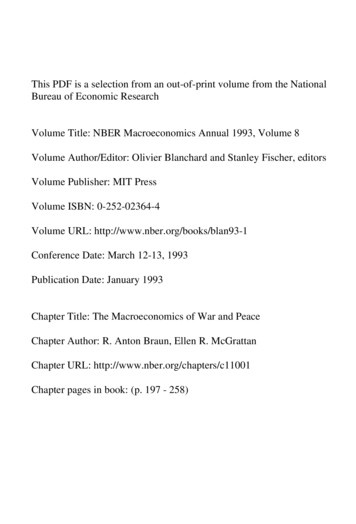
Macroeconomicsof War and Peace ? 207and Sylla (1991) report that nominal yields on consols rose steadily during the war from 3.46% in 1914 to 4.62% in 1919. Similarly, governmentissues rose from 3.96% in 1914 to about 6% in 1920. However, theseincreases in nominal yields were small relative to the price increasesdocumented earlier. After accounting for the effects of inflation, ex postreturns are negative for the duration of the war.2.2 THE UNITEDSTATESECONOMYDURINGWORLDWAR IThe outbreak of war in Europe caused financial panic in the UnitedStates. The U.S. stock market suspended operations on July 31, 1914,to avoid facing an onslaught of panic sell orders from Europe. Expectations that trade flows would be disrupted produced steep declines incommodity prices for cotton and wheat. The prices of many other tradedgoods like copper, steel, meat, and oil fell as well. In contrast to theEuropeans who placed embargoes on exports of gold at the outbreak ofwar, the United States continued to honor its gold obligations. Theinitial panic in the United States subsided rapidly as it became clear thatthe war would increase demand for many U.S. goods. After the UnitedStates entered the war in April 1917, further disruptions occurred asthe country mobilized for war. The Armistice was signed on November11, 1918, nineteen months after the United States' entry into the conflict.2.2.1 U.S. GNP and its ComponentsDuring World War I The U.S. experience in World War I was similar to the British experience in many respects. The lower plot in Figure 1 displays the shares of the expenditurecomponents of GNP. As in Britain, World War I produced majorchanges in the composition of output. While the magnitude of the U.S.war effort was much smaller than in Britain, the pattern of responses ofconsumption and investment were quite similar. Increased governmentspending acted to crowd out private consumption and investment. Netexports, which were negative in 1913, rose rapidly after the outbreak ofhostilities and peaked at 6% of GNP in 1916.In the course of the war, the U.S. government devoted a small, butsignificant, fraction of its expenditures to activities that expanded thecountry's productive capacity. The disruption of trade flows in Europeand the neutrality of the United States created a demand for U.S. goodsthat quickly absorbed the resources of the entire U.S. merchant shippingfleet. To help meet the shortage of merchant shipping, the United StatesShipping Board was established. The goal of this government enterprisewas to provide a supply of merchant vessels that could support navalforces in the case of war and facilitate foreign commerce with otherneutral countries. By the end of the war, the government had signed

208 ?BRAUN & MCGRATTANcontracts to build 3,116 freighters with a deadweight tonnageof 16,914,047 tons. This was equal to one third of the world merchant tonnage in 1913 (Crowell, 1920). As of December 31, 1918, 2,769,337,500 had been authorized for ship construction under thisprogram. This amount was twice the navy's ship building budget andabout 4% of GNP in 1918. The U.S. government made further investments in munitions and industrial plants of about 600 million, and sold 2.2 billion of trucks and buses (original cost) after the war (Cook, 1948).2.2.2 The U.S. Labor Market During World War I Panel A of Table 2contains information on aggregate labor market statistics for the UnitedStates during World War I. Consider the patterns in civilian employment. Kendrick's measure of persons engaged increases from 1914through 1917 and then declines in 1918, the year that conscriptionreached its peak. This pattern is different from Britain, where civilianemployment dropped steadily throughout the entire war. One reasonfor this difference is the smaller migration of manpower into the armedservices. At their peak the U.S. armed forces were only 65% of thesize of the British forces. Table 2 also contains Kendrick's measure ofman-hours divided by the population over 16. This measure shows anincrease in labor input during World War I. Kendrick's measure of laborproductivity is listed in column five. Labor productivity declines in 1917and then recovers in 1918. Once trend growth is taken into account,these data show no strong pattern in labor productivity during WorldWar I. Finally, note that real wages are basically constant until 1917,and then increase in 1918-1920.2.2.3 Prices in the U.S. During World War I The evolution of prices inthe United States during the war is similar to patterns already documented in Britain. Between 1913 and 1918, the CPI increased by 57%and by 1920 prices had risen by 133%. These increases are on a comparable scale with the British experience, although U.S. prices started risingsomewhat later than in Britain. Commodity prices in the United Statesalso closely mimic the evolution of British prices for comparable items.Commodity prices rose by 110% between 1913 and 1918. In both countries the sharpest increases in commodity prices occurred in 1916 and1917 and then stabilized in 1918 as government price controls wereextended.Price controls were put into effect shortly after the United States entered the war in response to rapidly escalating prices. For instance, steelplates doubled in price during the first five months of war and food

Macroeconomicsof Warand Peace?209prices rose by 28% over the same period (see Mitchell, 1919). Pricecontrols on food were effected by licensing requirements. Licenses wererequired for merchants who imported, manufactured, stored, or distributed specific items. Farmers, gardeners, and small businesses were exempted. Penalties were set for hoarding goods, destroying goods withthe intent to drive up prices, or making excessive profits. Violators weresubject to fines ranging from 5 to 10,000, the revocation of their licenses, and jail sentences for serious violations (Mitchell, 1919). In practice prices were not directly fixed: Rather markups were limited by"reasonable margin-of-profit" rules. Reasonable profit margins were initially based on prewar profit margins, but, as the war advanced, thiswas replaced by a two-tier system with distinct margins for high-costand low-cost dealers. While price controls led to shortages of some items(e.g., sugar), a formal system of rationing was not used for consumeritems in World War I. Instead the government relied on appeals todealers to limit sales to each customer of items in short supply (Rockoff,1984).Wage controls were not applied in the United States during WorldWar I. Instead the government took an active role in matching workerswith employers and mediating labor disputes. In a few rare instances,the government seized key industries where labor problems were particularly acute. The most notable example was Smith and Wesson. Labordisputes also played a role in the government's decision to take overthe railroads.Taken together these measures were largely successful in bringinginflation under control by the beginning of 1918 (Rockoff, 1984, p. 69).2.2.4 U.S. Financial Markets During World War I One result of war inEurope was that New York assumed London's position as the leadingcenter of international finance. European powers floated large loans inthe United States during the war, and by the war's end nearly half ofthe world's gold reserves were located in the United States. In the period from 1915 to 1917, (nominal) yields on bonds tended to decline(Homer and Sylla, 1991). However, the U.S. entry into war produced adecline in the bond market. Yields on prime corporate debt rose from3.98 to 4.98% between January and October 1917. Commercial paperrates rose from 3.84% in 1916 to 5.07% in 1917. Yields on Liberty government bonds, which were tax exempt, rose quickly after their issue at3.5% to 3.61%. These yields appear to be low given the rapid escalationof prices during this period. Ex post real rates on commercial paperwere negative between 1915 and 1917 and in 1919.

Table 2EMPLOYMENT, HOURS, PRODUCTIVITY, AND WAGES IN THE U.S. DURWORLD WAR IIA. World War nds)Man-hoursper capitac(1913 ,8971,173343100969499100989495Laprodu(191311111

B. World War ands)Man-hoursper capitac(1941 1941 8991010101011aKendrick'smeasure of persons engaged as reportedin LongTermEconomicGrowth(1973,p. 194).bArmed forces from Historical Statistics of the U.S., U.S. Department of Commerce (1975, p. 1141).'Kendrick'stotal private man-hoursas reportedin LongTermEconomicGrowth(1973)divided by populationover 1dKendrick'sindex of output per man-houras reportedin LongTermEconomicGrowth(1973).eRealwages in manufacturingdefined as the ratio of average hourly earnings in manufacturingfrom HistoricalStby the CPI all items same source, p. 211.

212 . BRAUN & MCGRATTAN2.3 A COMPARISONOF U.S. AND BRITISHEXPERIENCESIN WORLDWAR IOur analysis of the British and U.S. economies shows three commonfeatures during World War I. First, the response of the major components of output was the same in both countries. The increased government demand for goods raised output and crowded out privateconsumption and investment in both countries. Second, significant fractions of government purchases were used to expand productive capacityduring the war. For example, in Great Britain, the government helpedfinance expansions to the steel industry. In the United States, the government took a lead role in expanding the merchant marine. Third,labor productivity increased in both coun

Chapter pages in book: (p. 197 - 258) R. Anton Braun and Ellen R. McGrattan . RESERVE BANK OF MINNEAPOLIS The Macroeconomics of War and Peace* 1. Introduction This paper examines the effects of government purchases on economic activity. . and financial markets. In Section 3, we describe a simple model that takes into ac- count government .