Transcription
Understanding SWR by ExampleTake the mystery and mystique out of standing wave ratio.Darrin Walraven, K5DVWItsometimes seems that one ofthe most mysterious creaturesin the world of Amateur Radio isstanding wave ratio (SWR). Ioften hear on-air discussion of guys bragging about and comparing their SWR numbers as if it were a contest. There seemsto be a relentless drive to achieve the mostcoveted 1:1 SWR at any cost. But why? Thisarticle is written to help explain what SWRactually is, what makes it bad and when toworry about it.What is SWR?SWR is sometimes called VSWR, forvoltage standing wave ratio, by the technicalfolks. Okay, but what does it really mean?The best way to easily understand SWR is byexample. In the typical ham station setup, atransmitter is connected to a feed line, whichis then connected to the antenna. When youkey the transmitter, it develops a radio frequency (RF) voltage on the transmissionline input. The voltage travels down the feedline to the antenna at the other end and iscalled the forward wave. In some cases, partof the voltage is reflected at the antenna andpropagates back down the line in the reversedirection toward the transmitter, much likea voice echoing off a distant cliff. SWR is ameasure of what is happening to the forwardand reverse voltage waveforms and how theycompare in size.Let’s look at what happens when a transmitter is connected to 50 Ω coax and a 50 Ωantenna. For now, pretend that the coax cabledoesn’t have any losses and the transmitteris producing a 1 W CW signal. If you wereto look at the signal on the output of thetransmitter with an oscilloscope, what youwould see is a sine wave. The amplitude ofthe sine wave would be related to how muchpower the transmitter is producing. A largeramplitude waves means more power. Thiswave of energy travels down the transmissionline and reaches the antenna. If the antennaimpedance is 50 Ω, just like the cable, thenall of the energy is transferred to the antennasystem to be radiated. Anywhere on thetransmission line you measured, the voltagewaveform would measure exactly the sameas the sine wave coming from the transmitter.This is called a matched condition and is whatTable 1SWR vs Reflected Voltageor ��ected (%)05913172023262931334350566782PowerReflected ns with a 1:1 SWR.For the case of resistive loads (see sidebar),the SWR can be easily calculated as equal tothe (Load R)/Z0 or Z0/(Load R), whichevergives a result greater than or equal to 1.0.The load or terminating resistance is theRF resistance of whatever is on the end ofthe transmission line. It could be an antenna,amplifier or dummy load. The line impedance is the characteristic impedance of thetransmission line and is related to the physical construction of the line. Conductor size,space between conductors, what plasticwas used in the insulation — all affect lineimpedance. Generally, the cable manufacturer will list the line impedance and there’snothing you, as a user, can do to change it.But, what if the antenna wasn’t 50 Ω?Suppose that the antenna is 100 Ω and theFigure 1 — A graph showing the additional loss in a transmission line due to SWRhigher than 1:1.From November 2006 QST ARRL
Adding Reactance to the PictureIn the main article I used several examples of SWRbased on a resistive load. A resistive load is the easiestto visualize, calculate and understand, but it’s not themost common type of load. In most cases, loads havesome reactive impedance as well. That is, they containa resistive part and an inductive or capacitive part incombination. For instance, your antenna might appearas a 50 Ω resistor with a 100 nH inductor in series, orperhaps some capacitance to ground. In this situation,the SWR is not 1:1 because of the reactance. Evenantennas that show a perfect 1:1 SWR in mid-bandwill typically have some larger SWR at the band edges,often due to the reactance of the antenna changing withfrequency. Fortunately, a given SWR behaves the sameon a transmission line whether it’s reactive or resistive. Ifyou have a handle on understanding the resistive case,the concept will get you pretty far.To explore SWR further, it’s useful to look at thereactive load case, or what happens under the conditionthat loads are not simply resistive. Complex imaginarynumber math is the routine way to analyze the SWRof complex loads and can be done if you have accessto a calculator or computer program that will handle it.Even so, the math gets tedious in a hurry. Fortunately,there’s a very easy way to analyze complex loads usinggraphical methods and it’s called the Smith Chart. SeeFigure A.The concept behind the Smith Chart is simple. Thereis a resistive axis that is down the middle of the chart,left to right, and a reactive axis along the outer edge ofthe chart’s circumference. Inductive loads are plottedin the top half of the graph, and capacitive loads in thebottom. Any value of resistance and reactance in aseries combination can be plotted on the chart. Then,with a ruler and compass the SWR can be determined.Advanced users of the chart can plot a load and usegraphic techniques to design a matching structure orimpedance transformer without rigorous math or computer. It’s a very powerful tool. Here’s a simple exampleshowing how to determine SWR from a known loadusing the chart.Suppose you have just measured a new antennawith an impedance bridge and you know that the inputimpedance is 35 Ω in series with 12 Ω reactive. Thecoax cable feeding it has a Z0 of 50 Ω. What is the SWRat the antenna end of the coax?This impedance can be written as the complex number Z 35 j12.5 Ω. The “j” is used to indicate the reactive part from the real part and they can’t simply addtogether. To use a “normalized” Smith Chart we dividethe impedance by 50 Ω, to normalize the impedance.[Smith Charts are also available designed for 50 Ω with50 at the center instead of the 1.0 that we show for thenormalized chart. — Ed.] We now have Z 0.7 j0.25.Smith Chart numbers are normalized, which means thatthey have been divided by the system impedance beforebeing plotted. In most cases, the system impedanceis the transmission line impedance and is representedon the chart by the dot in the center. Now plot Z on thechart. Along the horizontal line find the 0.7 marker andmove upward (inductors or positive reactances areupward, capacitors or negative reactances are downFrom November 2006 QST ARRLFigure A — The normalized Smith Chart, ready to simplifytransmission line analysis.Figure B — An impedance of 35 j12.5 Ω normalized to 0.7 j0.25 Ωto use on the normalized chart.
Figure C — A circle of constant SWR drawn through the impedanceof Figure B. The SWR is 1.6.Figure D — A line drawn from the chart center through theimpedance of Figure B to the edge showing the distance from thepure resistive points on the line.ward from center) until you cross the 0.25 reactance line(see Figure B). Draw a point here that notes your impedance of 35 j12.5 Ω. Next draw a line from the centerdot of the chart to your Z point. Measure the distance ofthat line, then draw the same length line along the bottom SWR scale. From here you can read the SWR forthis load. The SWR is 1.6:1.Another useful attribute of the Smith Chart is calleda constant SWR circle. The SWR circle contains allthe possible combinations of resistance and reactancethat equal or are less than a given SWR. The circlesare drawn with a compass by using the distance fromthe SWR linear graph at the bottom and drawing acircle with that radius from the center of the chart, oruse the numbers along the horizontal axis to the rightof the center point. For instance, where you see 1.6 onthe horizontal line, a circle drawn with radius distancefrom the center to that point is SWR 1.6:1 as shown inFigure C.Now, any combination of impedance on the circle willbe equal to SWR 1.6:1 and anything inside the circle willbe less than 1.6:1. The example impedance that wasplotted before should lie on the 1.6:1 circle.Also useful is to know that rotating around the outerdiameter of the Smith Chart also represents a halfwavelength of distance in a transmission line. That is, asyou move along the outer circle it’s the same as movingalong a transmission line away from the load. One timearound the circle and you’re electrically λ/2 away. Thisis also very powerful feature of the chart since it allowsyou to see how your load impedance changes along atransmission line again, without doing the math.Here’s another example. If your coax cable has a1.6:1 terminating SWR, as you move along the transmission line away from the load, you move along theconstant SWR circle on the chart. Remember from thearticle text that a 1.6:1 SWR can be equal to either80 Ω or 31 Ω resistive? (1.6 80/50 or 50/31) From theSmith Chart, where the SWR circle crosses the horizontal axis, the impedance is purely resistive! Wherethe circle crosses 1.6, it’s equal to 80 Ω and crossing at0.62, it’s equal to 31 Ω. This is the basis of how impedance transformers work. Remember to multiply anynumbers from the chart by your working impedance(50 Ω in this example) to get their actual value.Where do these purely resistive points lie on thetransmission line? From the chart, looking at the lineextended from the center dot through our Z point, findwhere it crosses the “wavelengths toward generatorcurve” on the outside of the chart as shown in Figure D.The line crosses at approximately 0.07 wavelengths onthe chart, which will be the starting point. Note that the80 Ω point (1.6) is at 0.25 λ and the 31 Ω point (0.62) isat 0.50 λ on the chart. Subtracting the starting point of0.07, the chart is telling us that at 0.18 λ (0.25 – 0.07)from the load, the impedance is 80 Ω and at 0.43 λaway, it’s 31 Ω.To find the distance in a real piece of cable, multiplythe chart wavelengths by the free space wavelength bythe cable velocity factor. For example, if your frequencyis 144 MHz then a full wavelength in air would be300/144 2.08 meters. Multiplying by the velocity factor of 80% gives 1.67 meters. Multiplying by the chartwavelengths and then at 30 cm, you’d find 80 Ω and at72 cm it’s 31 Ω.From November 2006 QST ARRL
wave. At some places on the cable the reflectied voltage adds to 133 percent, and othersit subtracts to 66 percent of the matchedtransmitter output. The voltage ratio is133/66 or 2.0. That voltage ratio defines theSWR. The fact that the voltage along the linechanges with position and is different fromwhat the transmitter would produce is calleda standing wave. Standing waves are onlypresent when the line is mismatched.Does Higher SWR Lead to LowerPower Being Transmitted?Not always so dramatically. Believe it ornot, 100 percent of the power is actually transmitted in both of the previous examples. In thefirst case, with a 50 Ω antenna, it’s easy to seehow all the power is transferred to the antennato be radiated since there are no reflections.In the second case, the 33 percent voltagereflection travels back down to the transmitterwhere it doesn’t stop but is re-reflected fromthe transmitter back toward the antenna alongwith the forward wave. The energy bouncesback and forth inside the cable until it’s allradiated by the antenna for a lossless transmission line. An important point to realizeis that with extremely low loss transmissionline, no matter what the SWR, most of thepower can get delivered to the antenna. A laterexample will show how this can happen.Is High SWR Bad, or Not?Now that you have a sense of what SWRis, a few examples can show why undersome conditions, high SWR can lead to lesspower radiating and in other cases, it’s nobig deal. The easiest way to see how SWRaffects an antenna system is to use a set ofcharts. Figures 1 and 2 are taken from TheARRL Handbook in the chapter discussingtransmission lines. There is much moretheory in the Handbook than I’m presentinghere, so if you want to be an expert on transmission lines, that’s one place to learn more.In the previous examples, the transmission line had no loss and all our powerwas being delivered to the antenna. That’sa nice way to visualize what is happeningwith the reflections, but it doesn’t match thereal world because all transmission linesFigure 2 — A graph showing the actual SWR at an antenna based on measured SWR athavesome loss. Here’s a more practical,the transmitter end of a transmission line with loss.straightforward situation. This time we havea length of 50 Ω cable with a total loss of3 dB (50 percent power), and a 50 Ω antenna.cable is still 50 Ω. The SWR for this setup is reflected for various SWR values.calculated as 100/50, or 2:1. Now the energyIn the case of a mismatched condition, SWR is therefore 1:1. Transmitting 1 Wwave hits the antenna and part of it is radi- something interesting happens along the would result in 0.5 W applied to the antenna.ated by the antenna, but part of it is reflected transmission line. Before, with the matched Since the SWR is 1:1 there is no mismatchback down the line toward the transmitter. antenna, the same voltage existed anywhere loss to worry about. A very simple situationThat is, the antenna is not matched to the line, along the line. Now as you move along the and no charts are needed. If life were onlyso there is a reflection. It turns out that for a distance of the line, the voltage will change. that simple!Next ryt het 100Ω antenna with het asme2:1 SWR, 33 percent of the voltage wave is It now has peaks and valleys. The 33 percentreflected like an echo back down the line. reflection from the antenna alternately adds coax. The SWR is then 2:1 at the antennaTable 1 lists how much voltage and power is to and subtracts from the forward voltage since 100/50 2.0. According to Figure 1,From November 2006 QST ARRL
expect a mismatch loss of 0.35 dB in addition to the cable loss. In this case we lose atotal of 3.35 dB of our signal and send theantenna 0.46 W. Not much difference froma perfect SWR of 1:1.How about a SWR of 3:1 with the samecable? According to Figure 1 again, we wouldhave an additional loss of 0.9 dB, whichmakes a total loss of 3.9 dB and 0.41 W tothe antenna. This is still not a lot of additionalloss even with an SWR of 3:1. Under mostconditions a power reduction of 0.9 dB is notnoticeable over the air. Even at a 3:1 SWR, thesignal it not significantly reduced.The SWR vs loss tables make it easy tofigure out what your additional loss might befor any given antenna system, as long as youknow the matched cable loss.Is that the Whole Story?No, not exactly. There’s even more toexplore in the world of SWR. One verystrange situation occurs on a long and lossytransmission line, which causes your SWRto appear good at your transmitter even if it’sterrible at the antenna. It’s entirely possibleto have a good measured SWR, huge lossesin your feed line and no power getting out.Here’s an example.You’ve just set up your new 2 meterantenna and are feeding it with 120 feet ofRG-8X cable. The manufacturer’s data saysyou should expect 4.5 dB of cable loss forthis length of cable at 2 meter frequencies.Not great, but you accept it. You measurethe SWR at your transmitter and record a 2:1,which isn’t great but not too terrible either.But wait — how bad is it? Remember allthose reflections bouncing back and forth inthe cable? Earlier I told you that they eventually radiate, but that was without cable loss.The story is different now — we have loss.Each one of the reflections is attenuated in thecable by 4.5 dB every time it goes from oneend to the other or 9 dB round trip. The cableloss is attenuating the reflections and they dieout in the cable instead of being radiated.So, how bad is it really? Take a look atFigure 2. With a SWR at the transmitter of2:1, and a 4.5 dB cable loss, the chart shows a20:1 SWR at the antenna! Wow! That’s muchworse than the 2:1 measured at the transmitter. Looking back at Figure 1, that 20:1 SWRat your antenna is costing you another 7 dBof mismatch loss. In reality, the antenna system that you thought has only 4 dB of losshas 11 dB. Less than 1/10th of your transmitter power is being radiated! Good grief!If this same cable had an open circuitinstead of an antenna, and was several hundred feet long, the SWR meter at the transmitter would read 1:1. Why? Because cable losstends to make a very long cable appear likea virtual resistance to the transmitter as thereflections die out in the cable. Remember, at him because you know that the 4500 Ω ofno reflections looks like a SWR of 1:1. The the antenna will present an SWR of 90:1 onvalue of that virtual resistance in this case is his 50 Ω cable resulting in a mismatch loss50 Ω which is the definition of characteristic of 12 dB beyond the 0.25 dB cable loss. Sureimpedance, or why some cables are called he can tune his SWR to 1:1 with the tuner50 Ω and some are 75 or 300 Ω. That num- at his radio, but guess who will be workingber is the impedance the RF would see if the the DX?cable were infinitely long. Or, it is also theresistance of the load needed in order to cause Conclusionno reflected energy and match the cable.I hope I have been able to show byThe moral of this story is to measure example that SWR can be a serious issue, orthe SWR at the antenna, especially if you something not so important. With the helphave a long cable run. SWR measurements of the graphs and a little information aboutat the transmitter can be deceiving. The your transmission line and antenna, it’s easysecond moral is to know that when a cable to determine how much of your signal ismanufacturer quotes loss numbers, they are actually getting on the air or how much isbased on an SWR of 1:1, or a perfect match. being lost in the transmission line.Anything less than a perfect match can cause Darrin Walraven, K5DVW, has been licensedadditional losses.since 1986 at the age of 18. He enjoys DX, CWand SSB. He has an engineering degree fromTexas A&M University and is employed as anRF design engineer. You may contact him atOpen wire line, window line or lad- k5dvw@hotmail.com.Why Ladder Line Works forHigh SWRder line has been used since the early daysof radio. There is a good reason, since theloss of this type of cable is quite low at HFfrequencies — lower than all but the verybest coax cable. For instance, 300 feet of450 Ω ladder line has a loss of less than0.5 dB at 30 MHz when matched. A goodquality expensive coax might have 1 dB ofloss in the same length, but most high endamateur coax cable will have more than 2dB attenuation under those conditions. It isbecause of this low loss that air dielectric (ormostly air in the case of window line) linecan be used effectively on antennas that havehigh SWR, if the matching is provided at thetransmitter. The lower loss of this type ofline allows most of the reflections to radiateinstead of being lost within the cable.One last example shows how this works.You have just installed a full wave HF dipole.To feed it, you use 300 feet of 450 Ω ladderline with a loss of 0.5 dB at 30 MHz. You’vemodeled your antenna for 10 meters andyou just happen to know that the impedanceis 4500 Ω. That corresponds to a SWR of4500/450 or 10:1 on your ladder line. Prettybad, right? Not so fast. Consulting Figure 1and knowing your matched loss is 0.5 dBshows an additional loss of 0.9 dB at anSWR of 10:1. The total loss of this antennasystem is 1.4 dB. Not bad. Toss in a balancedline tuner and you’re ready to go!Your smart aleck buddy decides to installthe same antenna but he springs for thebest and most expensive coax figuring hisantenna is only 40 feet away from his radioand he doesn’t like the look of ladder line.He boasts that his coax loss is specified at0.25 dB, which is half that of your ladderline. He figures he can also use a tuner totake care of the mismatch. You quietly smileNew ProductsUNIVERSAL DIGITALDIAL FROM ELECTRONICSPECIALTY PRODUCTS The Model DD-103 Universal DigitalDial adds a digital frequency displayto vintage receivers. It counts onlythe VFO (local oscillator) signal, andVFO offset and band information formany receivers is stored in the display’smemory. A manual program modeallows programming up to 32 bandsfor any receiver that’s not included onthe preprogrammed list. Each band canbe individually calibrated to allow forcrystals that have aged or any other misalignment or error, to a rated accuracy of10 Hz. Calibration information is alsostored in memory, so each band only needsto be calibrated one time. The DD-103can also serve as bench frequency counterup to 40 MHz. Power is from the receiver,and power and signal cables are supplied.The complete instruction manual, a listof preprogrammed receivers and currentpricing information is available online atwww.electronicspecialtyproducts.com.From November 2006 QST ARRL
If you have questions for us, ARRL can be reached by phone during business hours, Monday through Friday, at 1-860-594-0200 or by email at membership@arrl.org. Please excuse us while we update our home page and membership management systems. We will be debuting our new look on Tuesday so please join us then.