Transcription
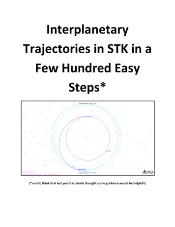
InterplanetaryTrajectories in STK in aFew Hundred EasySteps*(*and to think that last year’s students thought some guidance would be helpful!)
Satellite ToolKit Interplanetary TutorialSTK Version 9INITIAL SETUP1) Open STK. Choose the “Create a New Scenario” button.2) Name your scenario and, if you would like, enter a description for it. The scenario time is not toocritical – it will be updated automatically as we add segments to our mission.
3) STK will give you the opportunity to insert a satellite. (If it does not, or you would like to addanother satellite later, you can click on the Insert menu at the top and choose New ) The OrbitWizard is an easy way to add satellites, but we will choose Define Properties instead. We chooseDefine Properties directly because we want to use a maneuver-based tool called the Astrogator,which will undo any initial orbit set using the Orbit Wizard. Make sure Satellite is selected in the leftpane of the Insert window, then choose Define Properties in the right-hand pane and click theInsert button.4) The Properties window for the Satellite appears. You can access this window later by right-clickingor double-clicking on the satellite’s name in the Object Browser (the left side of the STK window).When you open the Properties window, it will default to the Basic Orbit screen, which happens to bewhere we want to be. The Basic Orbit screen allows you to choose what kind of numericalpropagator STK should use to move the satellite. Since we want to perform maneuvers, chooseAstrogator from the Propagator pull-down menu. This changes the Basic Orbit window to look likethe one below.
5) Notice at the top that the Central Body is the Earth. This is good since we are starting at Earth. Ifyou were modeling only heliocentric orbits or those about other planets, you could change thecentral body for the scenario by making sure that “Planetary Options” is checked on the View menuat the top of the STK window, then using the pull-down on the New Scenario button at the top leftof the STK window to create a new scenario around a different central body.6) Set the Initial State of the satellite to be the initial circular orbit. You can do this most easily byselecting Keplerian in the Coordinate Type pull-down menu. Set an initial circular orbit (Eccentricity 0) with a 300 km altitude (Semi-major Axis 6678 km). The Inclination should be 28.5 degrees,and probably already is by default. The Orbit Epoch time at the top tells you at what time thesatellite will have the True Anomaly specified at the bottom.7) The left pane of the Basic Orbit window lists the pieces of your trajectory, called Mission ControlSegments, or MCS. After the Initial State, there should already be a segment called Propagate. Clickon the Propagate segment.
8) The first option available to you is which type of propagator to use to numerically integrate theequations of motion. Click the “ ” button next to the Propagator name to choose from theavailable options. To match the calculations you have done by hand, choose Earth Point Mass asyour propagator. (The others will include contributions from the oblateness of the Earth orgravitational effects from third bodies and will show how your orbit would drift given these effects.)9) There are many options for how long to allow the satellite to continue in its original orbit. These arecalled Stopping Conditions. Time is always selected by default, and is always set to 43200 seconds,or 12 hours. Click the Insert button next to Stopping Conditions to choose other options.
10) If you want to allow the satellite to orbit three times before performing its next maneuver, a goodstopping condition is counting how many times the satellite passes the Ascending Node. ChooseAscendingNode from the Stopping Conditions list, and click OK.11) Now your Propagator window has two Stopping Conditions. Click the line for Duration, then theRemove button. (You must always have at least one stopping condition, so you cannot remove theDuration condition until you add another one.)12) Underneath the list of Stopping Conditions is an area where you can set the details of the stoppingcondition. To allow the satellite to pass the ascending node three times, change the number in theRepeat Count box from 1 to 3.
13) The color next to the word Propagate in the left pane shows the color that the orbit will be in thegraphics window for that segment. It is a good idea to make each segment a different color so thatyou can identify the segments easily in the graphics window. Double-click on the word Propagate tobring up a screen that allows you to change the color. For practice, change the color of the firstsegment to white.14) Click the button with the green arrow, just above the left pane, to run the mission control sequencesthrough the Astrogator, then click OK to return to the main window.15) If the Insert STK Objects window is still open, you can close it. You can also close the 2D graphicswindow and focus on the 3D graphics window. You should see your satellite’s initial orbit circlingthe Earth. You can click the blue arrow at the top of the window to see your satellite moving. Youcan left-click the mouse and drag to move the planet in the window. You can right-click and drag tozoom in and out. You can use the view buttons at the top of the 3D graphics window (look like eyes)to switch to preset views.16) This is an excellent time to save your Scenario. STK saves a set of several files, called a Scenario, somake a folder for this particular Scenario and save it somewhere you can find it.
CHANGING TO THE ECLIPTIC PLANE17) The first maneuver in the interplanetary trajectory is to change planes from the initial orbit plane tothe ecliptic plane (the plane of the Earth’s orbit about the Sun). This would be easier to visualize ifwe could see the ecliptic plane. Good news! STK can do that. Select the 3D graphics window. Atthe top of the window, select the Properties button.18) Take a few minutes to look through the options available to you. In the Details window, you canturn on the Equator, to help highlight the inclination of the orbit. In the Grids window, you can turnon the ecliptic plane by selecting the Show checkbox under Ecliptic Coordinates. In the Vectorwindow, you can turn on a vector that shows the Vernal Equinox direction from which rightascensions are measured. (If you turn this vector on, you have other options, like “Draw at CentralBody” and “Show Label,” both of which make sense. You can also choose a color for the axis.) Inthe vector window, you can also choose the “Add” button to add other vectors you might finduseful, such as a vector showing the normal direction to the ecliptic plane. For now, turn on theecliptic plane grid and the Vernal Equinox vector.19) Click OK to return to the 3D graphics window. Notice that the orbit passes through the vernalequinox vector, since the default right ascension in the Astrogator initial state was 0, and we
didn’t change it. You can experiment with different right ascensions to see how much plane changewill be required to move from the initial orbit into the ecliptic plane.20) With 0,you can see from the 3D graphics window that the plane change should take place whenthe satellite crosses the equator, since this is a point common to both the original orbit plane andthe ecliptic plane. Conveniently, we are already propagating the initial orbit to a crossing of theequator (Stopping Condition AscendingNode), so we are set to perform our plane change after thesatellite goes around the Earth a few times. Double-click on the satellite’s name to open theAstrogator window.21) Insert a new Mission Control Segment in the left pane by right-clicking on the blue arrow andchoosing Insert Before. You can also insert a segment by clicking the button that looks like a blanksheet of paper, just above the left pane.22) Take a minute to look at the segments that are available to you. Choose Maneuver and click OK.23) The Maneuver segment allows you to add rocket burns. You can choose Impulsive or Finite burns(we want Impulsive), how the rocket fires (Attitude tab), and even attributes of a specific engine, ifyou have that information. In the Attitude tab, click on the Attitude Control pull-down. Youroptions are:Along Velocity Vector -- delta-V vector is aligned with the spacecraft's inertial velocityvector (speed up).Anti-Velocity Vector -- delta-V vector is opposite to the spacecraft's inertial velocityvector (slow down).Attitude -- Attitude is defined using Euler Angles or a Quaternion.File -- Import an attitude file to set the maneuver.Thrust Vector -- The total delta-V can be specified in cartesian or spherical form withrespect to the thrust axes.We want to specify a delta-V that is out of plane, so choose the Thrust Vector option.24) Now you need to tell STK how much delta-V you want and in what direction. First, choose thrustaxes. Not sure what the axes mean? Click the “ ” button to bring up the Select Reference Axeswindow and see the options. Select any axes that look interesting and click the “Info ” button tosee how they are defined. For now, stick with VNC (Earth), so that the x-direction is aligned with thevelocity and the y-direction is normal to it (since we want our plane change delta-V to be normal tothe direction of motion).25) Return to the Basic Orbit page to finish specifying the plane-change maneuver. Calculate thenecessary delta-V for a simple plane change. Recall,
The ecliptic plane is inclined 23.43 from the Earth’s equatorial plane. Depending on the rightascension of the initial orbit, the plane change angle θ could vary from 23.43 -i0 to 23.45 -i0,where i0 is the inclination of the parking orbit.Calculation:θ Direction positive y or negative y?26) Enter the correct magnitude and sign for the plane change in the Astrogator screen. You may clickthe green arrow to apply the impulse.27) If you run the scenario now, it will look exactly the same as before, because there is no propagationafter the impulse to show the new orbit. Insert a Propagate MCS after the Maneuver. Allow thespacecraft to circle the Earth a couple of times on its new orbit, using the Earth Point Masspropagator and the AscendingNode stopping condition (and removing the Duration stoppingcondition). Make the new orbit a different color, such as red.28) Click the green arrow to run the Astrogator sequence. Look at the 3D graphics window, and you willnow see a red circular orbit aligned with the ecliptic plane grid. Run the simulation and watch yourspacecraft change planes.
29) Save your scenario.ALLOWING STK TO CALCULATE THE PLANE CHANGE FOR YOU30) Since STK can perform analysis in addition to creating visualizations of known orbits, you can use STKto calculate the required plane change delta-V for you. To try this, right-click on the satellite namein the Object Browser on the left of the screen and choose Copy. Right-click on the scenario name inthe Object Browser and choose Paste. You should now have two satellites: your original satelliteand one with the same name with a “1” at the end of it. Change the name of the new satellite toTargeterPractice.31) Double-click on TargeterPractice in the Object Browser to open the new satellite’s Astrogatorwindow. It should look just the same. Delete the plane change Maneuver by selecting it andclicking the red “X” button just above the MCS pane.32) Insert a new MCS segment between the two propagators. This time, choose Target Sequenceinstead of Maneuver.33) Click the plus sign next to the Target Sequence to expand it. You will see a blue arrow just like in thelarger Mission Control Sequence. Insert a Maneuver just above the Target Sequence’s blue arrow.34) Just as before, choose Impulsive for Maneuver Type and Thrust Vector for Attitude Control. Thewindow looks just as it did before except that now the boxes where you could enter delta-V valueshave little target icons next to them. Click the target icon next to the Y (Normal) delta-V box andnext to the X (Velocity) delta-V box. This sets the X and Y delta-Vs as independent variables that STKwill vary to try to accomplish goals that you will set for it. (Why include X? We have made theassumption in class that the delta-V is directly perpendicular for a simple plane change. Now we cansee how accurate that assumption was.)35) The goal is to change the orbit plane to the ecliptic plane. To tell STK this, click the “Results ”button under the MCS pane. There are many options to select for goals. We want to change theinclination, so expand the choices for Keplerian Elems and choose Inclination. Click the blue arrow to add the Inclination to the list of goals. Click OK to close the Results window.
36) The Results window allowed us to choose our variables. Now we need to set desired values. Clickon the Target Sequence in the MCS pane. On the right side is a box called Profiles. Highlight thedefault search profile, a differential corrector, and click the Properties button.37) Click the “Use” button next to the independent variables (X- and Y-components of the delta-V) andnext to the dependent variable (Inclination) so that the targeter knows to use them. Double-click inthe DesiredValue column and change the desired value of the inclination to 23.43 .
38) Click on the Convergence tab to view the options available to you. If you don’t see the results youwant after running the targeter, you can increase the number of iterations. For now, set it to 50iterations. It is a good idea to leave the “Display Status” box checked so that you can see what isgoing on. Click OK to return to the Astrogator window.39) In the Target Sequence window, change the pull-down menu on the upper right, for the Action, to“Run Active Profiles.” This turns the targeter on and allows it to run.40) Change the color for the final Propagate segment to a different color, say, pink, so that you can seethe two different trajectories (which will hopefully be quite similar).41) Click the green arrow to run the MCS.42) A window should open showing the results of the targeter. The delta-V applied is under the column“New Value.” The “Last Update” column shows how much the delta-V value was changed duringthe last iteration, and the “Difference” column shows the difference between the desired value andthe achieved value. You can use the information to decide whether you need to run the MCS again
(click the green arrow in Astrogator to have STK perform another 50 iterations using the last value asthe new starting value), increase the number of iterations, etc.43) The 3D graphics window will now display both orbits (one with the delta-V specified and one withthe delta-V found through the targeter), although you might have to zoom in quite closely todistinguish the two from each other.44) Experiment with changing the Tolerance for the dependent variable in the Properties window of theDifferential Corrector profile. An accuracy of 0.1 degrees might not be enough when propagatingout to other planets. Try 0.01 and see how much the delta-V changes.EARTH ESCAPE45) For now, close all of the TargeterPractice windows and double-click on the original satellite. We willadd an Earth-escape delta-V that will get us to a fly-by of Mars.46) The magnitude and location of this impulse was calculated in class (see pages 15-5 through 15-7 inthe Spring 2010 notes). The maneuver required an in-track delta-V of 3.55 km/s relative to theEarth, located at an angle of 29.2 below the vector of the Earth’s motion around the Sun.47) First, let’s create a 3D graphics window that looks the way we would draw an Earth-escapetrajectory. From the View menu at the top of the STK window, choose Duplicate 3D GraphicsWindow.48) Now that we have multiple graphics windows, it helps to givethem useful names. Click on the Properties icon for one ofthem. Choose Window Properties and call the first one PlaneChange View. Close that Properties window.49) Open the Properties for the new graphics window. UnderWindow Properties, rename it Earth Escape View. Click “Apply,”but leave the Properties open (or re-open the Properties if youclicked OK already).50) In the Vector part of the Properties, select the Show box next toEarth Sun vector. This will add a vector to your view that alwayspoints from the Earth to the Sun.51) Click Add to get a list of other possible vectors. Expand the listnext to Earth and choose “Velocity.” Click the arrow to add it tothe list at the right, then click OK.52) Click the checkbox to Show the Earth’s velocity vector. Choosea color for it and check “Show Label” so that you know what itis.
53) Click OK to close the graphics window Properties.54) To change the view so that you are looking directly down at the ecliptic plane, click the small eyeshaped icon with an arrow at the top of the 3D graphics window to open a window called ViewFrom/To.55) In the From window on the left, expand the vectors. You will likely have to add a vector, so click thegreen single arrow between the From and To boxes. Expand the options next to Earth, and chooseEclipticNormal. This will allow us to look straight down along this normal vector to the eclipticplane. Click OK to return to the From/To window.56) In the View From/To window, click Inward so that we are looking down on the ecliptic plane in theway we are used to drawing this plane. Click OK, and you will be able to see the new view in thebackground.57) Find the eye-shaped icon with the small arrow and cylinder at the bottom that takes you to StoredViews. Click on the arrow to expand it, then “Stored Views ” Click New to store this view so that
you can easily return to it if you drag around the window. Give it a useful name like EclipticNormalby double-clicking on the View Name and typing a new one.58) Double-click on the original satellite to open the Astrogator window so that we can add the Earthescape delta-V maneuver to our satellite.59) Click on the final Propagate segment. Rather than stopping when we cross the Earth’s equator, wewant to stop propagating along the ecliptic plane circular orbit when the satellite is 29.2 below thetail of the Earth’s velocity vector. STK can use the angle between two vectors as a stoppingcondition, if we tell it which vectors to use.60) In the Astrogator window, click on the button on the right-hand side of the second row of buttons(circled below) to open the Astrogator browser (also called Component Browser). You can alsoreach the browser from the Utilities menu by choosing Component Browser.61) In the Component Browser, expand the plus sign next to Calculation Objects, since we want to do acalculation, and choose Vector because we want to calculate the angle between two vectors.62) There is already a template called Angle Between Vectors. Click on it, and then click the Duplicatebutton toward the top of the window. The templates are saved as read-only files. Once youduplicate one, the icon changes colors from orange to green, and you can edit information likewhich vectors to use.
63) Give your new calculation object a useful name like “Angle Between Vectors – Earth Escape” so thatyou will remember what it is for when you see it later. You can add a description that tells you it isthe angle between the Earth’s velocity vector and the satellite’s position vector (which we will makeofficial in a moment). Click OK.64) Double-click on the name of the object you just created. You will see a window much like the onebelow, but you need to set the vectors to use. Double click in the Value column next to Vector1 toopen a list of known vectors. Expand the list for the Earth and choose Velocity. Double click in theValue column next to Vector 2. Expand the list for the satellite, and choose position.65) Click OK to close the window above, then again to close the Component Browser. Now we canreturn to the Astrogator and use this new stopping condition.66) In the Propagate segment, Click Insert to create a new stopping condition.67) Choose UserSelect from the available options and click OK to return to the Astrogator.68) To tell STK which user selected criterion to use are, click the “ ” next to User Calc Object. Thisopens a window called User Calculated Object Selection.69) Scroll toward the bottom of the options. Expand the plus sign next to Vector and choose AngleBetween Vectors – Earth Escape object that you just created. Click OK.
70) In the Astrogator window, set the Trip value (the value of the angle between the vectors that “trips”the stopping condition) to 150.8 . (We subtract the 29.2 from 180 because we were reallymeasuring from the negative of the velocity vector in the notes to get 29.2 . The 150.8 measurement is what we were calling η.)71) Next to the Trip value, you have the option (Criterion) for whether you want the propagator to stopwhen it reaches the specified angle as that angle is increasing, decreasing, or either. Since thesatellite is moving toward the velocity vector, set the Criterion to stop when the angle is decreasing.72) Remove any other stopping conditions in this segment and click the green Run button.73) Look at your Earth Escape View 3D graphics window. Does the red segment stop where you thoughtit should? (Note: if you want the satellite to orbit the earth completely one or more times, you canincrease the Repeat Count in the Propagator segment.) It will be even easier to see once you addthe Earth-escape delta-V.74) Return to the Astrogator. Insert a Maneuver after the last Propagate segment. Add an impulsivethrust along the velocity vector. Use the Attitude Control option called “Along the Velocity Vector”to simplify the input over using the Thrust Vector.75) Insert a Propagate segment after the Maneuver using a different color, say, light blue. For now, setthe stopping condition as the Earth’s sphere of influence radius, 9.24 x 10⁵ km by inserting an “R
Magnitude” stopping condition and setting the Trip condition to the sphere of influence radius. Usethe Earth Point Mass propagator again so that your simulation matches your calculations.76) Since you now have multiple maneuvers and propagation segments, rename them to somethingmeaningful by double-clicking (or single-clicking and hovering) and typing the new name. You canchange the color of the maneuvers to match the propagation segments in the list, but the maneuvercolors don’t show up in the 3D view like the propagation segments do. When you are done with therenaming, your Astrogator window will look something like this:77) Click the green arrow to run the sequence.78) Return to your Earth Escape View. Do you see the trajectory heading away from the Earth with anasymptote aligned with the Earth’s velocity vector? You might need to zoom out to see theasymptote.79) Save your scenario.
OUTSIDE THE EARTH’S SPHERE OF INFLUENCE – HELIOCENTRIC TRAJECTORY80) Within the same scenario, we can show the satellite’s orbit around the Sun after it leaves the Earth’ssphere of influence. First, let’s create a heliocentric view. From the View menu at the top of theSTK screen, choose New 3D Graphics Window.81) If the new window doesn’t have the usual set of toolbars across the top, right-click in the newwindow and choose 3D Graphics from the list of available Toolbars.82) On the right side of the Toolbar is a blue sphere-shaped icon with an arrow. Click on it to display alist of central bodies. Choose the Sun from the list.83) Open the Properties for the new 3D graphics window. In the Window Properties, rename thewindow “Heliocentric.” Click Apply.84) In the Advanced area, change the Max Visible Distance. By default, STK will show 1e 007 km in agraphics window. If you zoom out to show more than that, the orbits disappear. Since this is a viewin which we want to show at least as far as the diameter of Mars’ orbit about the Sun (4.558 x 10⁸km) and have room around the edges, change the Max Visible Distance to 1e 010 km. Click OK.85) If you zoom out far enough, you will be able to see the Moon, since it is turned on by default. Wearen’t particularly interest in the Moon, but we would like to be able to see Earth and Mars, and oursatellite.86) To turn off the Moon’s label: in the 3D graphics window, right click and add the Globe Managertoolbar. Click the first icon to turn on the Globe Manager, a small window under the Object Browseron the left side of your screen. Find the Moon and rick-click on it. Uncheck the Label option. Youcan close the Globe Manager.87) Click on the name of scenario in the Object Browser and open its Properties. Setting Properties atthe Scenario level will keep us from having to set the same options multiple times.88) We are interested in the 2D Graphics Global Attributes part of the Properties window. Even thoughwe are viewing 3D graphics windows, most STK objects (satellites, planets, etc) use the 2D graphicssettings to determine what is shown and how it looks.89) On the right side of the 2D Graphics Global Attributes window is a box labeled Planets. We want thefirst three items checked: Show Orbits allows us to insert planets and show a complete orbit foreach one; Show Inertial Positions marks the position of a planet with a dot; and Show PositionLabels puts the name of the planet next to the planet position dot. We want the last two itemsunchecked: Show Subplanet Points would put a point on the Sun underneath the planet, and ShowSubplanet Labels would put a label next to the point. The last two options can be confusing, makingit look like the planets are in the Sun if the window isn’t zoomed out far enough.
90) Click OK to apply the changes to the scenario and close the Properties window.91) To insert a planet, go to the Insert menu at the top and choose Object Catalog. Click on the Planetand choose Insert. You do not need to change the central body pull-down at the bottom. Do thistwice, since we want to insert both Earth and Mars.92) In the Object Browser, open the Properties for the first planet. In the Basic Definition, set thecentral body to Earth. Make sure that Auto-Rename is checked, and STK will automatically renamethe planet “Earth.” Click OK to close the window.93) Repeat the step above for the second planet, setting its central body to Mars. In the 2D Graphicsproperties for the planets, you can change the colors of the orbits if you wish.94) In the Heliocentric 3D graphics window, click the View From/To icon. As before, add a vector to theSun’s list of vectors that is the Ecliptic Normal. Set the view to be inward along this normal. Returnto the 3D window and zoom out until you can see both planets’ orbits. Save this view for laterconvenience.95) Save your scenario.96) Open the Astrogator for your satellite.97) Add a new Propagate segment to the bottom of your MCS list. Call the new segment Heliocentricand give it a new color.98) Change the Propagator for this segment to Heliocentric.99) Insert a stopping condition called Apoapsis that will stop the propagation at the point that thesatellite is farthest from the central body.100) Change the Central Body for this propagation by clicking the “ ” button next to the Central Bodybox in the area beneath the stopping condition. Select the Sun from the list of central bodies.101) Remove the Duration stopping condition and run the MCS by clicking the green button. Go toyour Heliocentric view. Did the satellite make it to Mars? Probably not. Does it even look like itreached an apoapse? Probably not. The reason is that STK sets a maximum amount of time that itwill propagate a segment, in case you set a stopping condition that can never be reached. Forexample, if I set as a stopping condition that STK should propagate until the satellite reachedJupiter, it would never happen. If STK didn’t have the propagation time safeguard, it would bestuck in an endless propagation loop.102) If you can’t see the satellite, go to its Properties page and open the 3D Graphics section. Click theModel option. Turn off the Detail Thresholds and turn on the Show box for showing the satelliteas a Point.
103) Return to the Astrogator. Next to box where you set the Propagator to Heliocentric is a buttonmarked Advanced. Click the Advanced button.104) Uncheck the box for Maximum Propagation Time and click OK.105) Run the MCS again. The Heliocentic view should now show half of a Hohmann ellipse.106) Run the scenario to the end, or if you just want to see the arrival point at Mars, copy the end timefrom the bottom-right of the last Astrogator propagation segment and paste in into the box forthe simulation time at the top of the graphics window. Unless you are very lucky, there will likelybe two problems with the arrival. First, Mars isn’t near the satellite at the end of the heliocentricpart of the satellite’s trajectory; second, the apoapse of the orbit doesn’t even line up with Mars’orbit, let alone its orbital position. The orbital position could be adjusted by changing the starttime of the simulation. The second problem occurs because we did our initial calculationsassuming that Mars’ orbit was circular and in the ecliptic plane, neither of which is entirelyaccurate. You can see the eccentricity of Mars’ orbit in the Heliocentric window by comparing itwith Earth’s which is more nearly circular. See how Earth’s orbit and Mars’ orbit are much closeron one side than the other?107) We will add a custom Mars in the next section. For now, save your scenario.CREATING A CUSTOM PLANETThis is a useful option for adding circular, elliptic plane pseudo-planets or for adding new central bodies,such as moons of the outer planets, that aren’t in the STK central body library.108) Open the Component Browser again from the Utilities menu.109) Click on the Central Bodies folder. Click on each of the listed central bodies and see if theDuplicate button at the top becomes non-gray. If it does, duplicate the body and skip the nexts
24) Now you need to tell STK how much delta-V you want and in what direction. First, choose thrust axes. Not sure what the axes mean? lick the " " button to bring up the Select Reference Axes window and see the options. Select any axes that look interesting and click the "Info " button to see how they are defined.