Transcription
This PDF is a selection from a published volume from the National Bureauof Economic ResearchVolume Title: The Economics of Artificial Intelligence: An AgendaVolume Authors/Editors: Ajay Agrawal, Joshua Gans, and Avi Goldfarb,editorsVolume Publisher: University of Chicago PressVolume ISBNs: 978-0-226-61333-8 (cloth); 978-0-226-61347-5 (electronic)Volume URL: http://www.nber.org/books/agra-1Conference Date: September 13–14, 2017Publication Date: May 2019Chapter Title: Artificial Intelligence and Behavioral EconomicsChapter Author(s): Colin F. CamererChapter URL: http://www.nber.org/chapters/c14013Chapter pages in book: (p. 587 – 608)
24Artificial Intelligence andBehavioral EconomicsColin F. Camerer24.1IntroductionThis chapter describes three highly speculative ideas about how artificialintelligence (AI) and behavioral economics may interact, particular in futuredevelopments in the economy and in research frontiers. First note that I willuse the terms AI and machine learning (ML) interchangeably (although AIis broader) because the examples I have in mind all involve ML and prediction. A good introduction to ML for economists is Mullainathan and Spiess(2017), and other chapters in this volume.The first idea is that ML can be used in the search for new “behavioral”type variables that affect choice. Two examples are given, from experimental data on bargaining and on risky choice. The second idea is that somecommon limits on human prediction might be understood as the kinds oferrors made by poor implementations of machine learning. The third ideais that it is important to study how AI technology used in firms and otherinstitutions can both overcome and exploit human limits. The fullest understanding of this tech- human interaction will require new knowledge frombehavioral economics about attention, the nature of assembled preferences,and perceived fairness.24.2Machine Learning to Find Behavioral VariablesBehavioral economics can be defined as the study of natural limits oncomputation, willpower, and self- interest, and the implications of thoseColin F. Camerer is the Robert Kirby Professor of Behavioral Finance and Economics atthe California Institute of Technology.For acknowledgments, sources of research support, and disclosure of the author’s materialfinancial relationships, if any, please see http://www.nber.org/chapters/c14013.ack.587You are reading copyrighted material published by University of Chicago Press.Unauthorized posting, copying, or distributing of this work except as permitted underU.S. copyright law is illegal and injures the author and publisher.
588Colin F. Camererlimits for economic analysis (market equilibrium, IO, public finance, etc.).A different approach is to define behavioral economics more generally, assimply being open- minded about what variables are likely to influence economic choices.This open- mindedness can be defined by listing neighboring socialsciences that are likely to be the most fruitful source of explanatory variables.These include psychology, sociology (e.g., norms), anthropology (culturalvariation in cognition), neuroscience, political science, and so forth. Call thisthe “behavioral economics trades with its neighbors” view.But the open- mindedness could also be characterized even more generally, as an invitation to machine- learn how to predict economic outcomesfrom the largest possible feature set. In the “trades with its neighbors” view,features are constructs that are contributed by different neighboring sciences.These could be loss aversion, identity, moral norms, in-group preference,inattention, habit, model- free reinforcement learning, individual polygenicscores, and so forth.But why stop there?In a general ML approach, predictive features could be—and shouldbe—any variables that predict. (For policy purposes, variables that couldbe controlled by people, firms, and governments may be of special interest.)These variables can be measurable properties of choices, the set of choices,affordances and motor interactions during choosing, measures of attention, psychophysiological measures of biological states, social influences,properties of individuals who are doing the choosing (SES, wealth, moods,personality, genes), and so forth. The more variables, the merrier.From this perspective, we can think about what sets of features are contributed by different disciplines and theories. What features does textbookeconomic theory contribute? Constrained utility maximization in its mostfamiliar and simple form points to only three kinds of variables—prices,information (which can inform utilities), and constraints.Most propositions in behavioral economics add some variables to thislist of features, such as reference- dependence, context- dependence (menueffects), anchoring, limited attention, social preference, and so forth.Going beyond familiar theoretical constructs, the ML approach to behavioral economics specifies a very long list of candidate variables ( features)and include all of them in an ML approach. This approach has two advantages: First, simple theories can be seen as bets that only a small number offeatures will predict well; that is, some effects (such as prices) are hypothesized to be first- order in magnitude. Second, if longer lists of features predict better than a short list of theory- specified features, then that findingestablishes a plausible upper bound on how much potential predictabilityis left to understand. The results are also likely to create raw material fortheory to figure out how to consolidate the additional predictive power intocrystallized theory (see also Kleinberg, Liang, and Mullainathan 2015).You are reading copyrighted material published by University of Chicago Press.Unauthorized posting, copying, or distributing of this work except as permitted underU.S. copyright law is illegal and injures the author and publisher.
Artificial Intelligence and Behavioral Economics589If behavioral economics is recast as open- mindedness about what variables might predict, then ML is an ideal way to do behavioral economicsbecause it can make use of a wide set of variables and select which onespredict. I will illustrate it with some examples.Bargaining. There is a long history of bargaining experiments trying topredict what bargaining outcomes (and disagreement rates) will result fromstructural variables using game- theoretic methods. In the 1980s there wasa sharp turn in experimental work toward noncooperative approaches inwhich the communication and structure of bargaining was carefully structured (e.g., Roth 1995 and Camerer 2003 for reviews). In these experimentsthe possible sequence of offers in the bargaining are heavily constrainedand no communication is allowed (beyond the offers themselves). Thisshift to highly structured paradigms occurred because game theory, at thetime, delivered sharp, nonobvious new predictions about what outcomesmight result depending on the structural parameters—particularly, costsof delay, time horizon, the exogenous order of offers and acceptance, andavailable outside options (payoffs upon disagreement). Given the difficultyof measuring or controlling these structural variables in most field settings,experiments provided a natural way to test these structured- bargainingtheories.1Early experiments made it clear that concerns for fairness or outcomesof others influenced utility, and the planning ahead assumed in subgameperfect theories is limited and cognitively unnatural (Camerer et al. 1994;Johnson et al. 2002; Binmore et al. 2002). Experimental economists becamewrapped up in understanding the nature of apparent social preferences andlimited planning in structured bargaining.However, most natural bargaining is not governed by rules about structureas simple as those theories, and experiments became focused from 1985 to2000 and beyond. Natural bargaining is typically “semi- structured”—thatis, there is a hard deadline and protocol for what constitutes an agreement,and otherwise there are no restrictions on which party can make what offersat what time, including the use of natural language, face- to-face meetingsor use of agents, and so on.The revival of experimental study of unstructured bargaining is a goodidea for three reasons (see also Karagözoğlu, forthcoming). First, there arenow a lot more ways to measure what happens during bargaining in laboratory conditions (and probably in field settings as well). Second, the largenumber of features that can now be generated are ideal inputs for ML topredict bargaining outcomes. Third, even when bargaining is unstructuredit is possible to produce bold, nonobvious precise predictions (thanks to therevelation principle). As we will see, ML can then test whether the features1. Examples include Binmore, Shaked, and Sutton (1985, 1989); Neelin, Sonnenschein, andSpiegel (1988); Camerer et al. (1994); and Binmore et al. (2002).You are reading copyrighted material published by University of Chicago Press.Unauthorized posting, copying, or distributing of this work except as permitted underU.S. copyright law is illegal and injures the author and publisher.
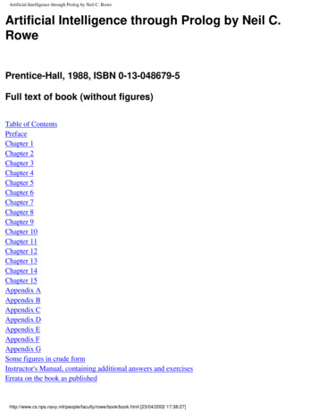
590Colin F. CamererFig. 24.1 A, initial offer screen (for informed player I, white bar); B, example cursor locations after three seconds (indicating amount offered by I, white, or demandedby U, dark gray); C, cursor bars match which indicates an offer, consummated at sixseconds; D, feedback screen for player I. Player U also receives feedback about piesize and profit if a trade was made (otherwise the profit is zero).predicted by game theory to affect outcomes actually do, and how muchpredictive power other features add (if any).These three properties are illustrated by experiments of Camerer, Nave,and Smith (2017).2 Two players bargain over how to divide an amount ofmoney worth 1– 6 (in integer values). One informed (I ) player knows theamount; the other, uninformed (U) player, doesn’t know the amount. Theyare bargaining over how much the uninformed U player will get. But bothplayers know that I knows the amount.They bargain over ten seconds by moving cursors on a bargaining numberline (figure 24.1). The data created in each trial is a time series of cursor locations, which are a series of step functions coming from a low offer to higherones (representing increases in offers from I) and from higher demands tolower ones (representing decreasing demands from U).Suppose we are trying to predict whether there will be an agreement ornot based on all variables that can be observed. From a theoretical pointof view, efficient bargaining based on revelation principle analysis predictsan exact rate of disagreement for each of the amounts 1– 6, based only onthe different amounts available. Remarkably, this prediction is process- free.2. This paradigm builds on seminal work on semistructured bargaining by Forsythe, Kennan, and Sopher (1991).You are reading copyrighted material published by University of Chicago Press.Unauthorized posting, copying, or distributing of this work except as permitted underU.S. copyright law is illegal and injures the author and publisher.
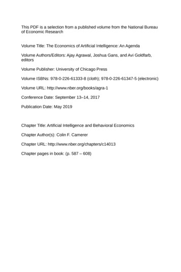
Artificial Intelligence and Behavioral Economics591Fig. 24.2 ROC curves showing combinations of false and true positive rates in predicting bargaining disagreementsNotes: Improved forecasting is represented by curves moving to the upper left. The combination of process (cursor location features) and “pie” (amount) data are a clear improvementover either type of data alone.However, from an ML point of view there are lots of features representing what the players are doing that could add predictive power (besides theprocess- free prediction based on the amount at stake). Both cursor locationsare recorded every twenty- five msec. The time series of cursor locations isassociated with a huge number of features—how far apart the cursors are,the time since last concession ( cursor movement), size of last concession,interactions between concession amounts and times, and so forth.Figure 24.2 shows an ROC curve indicating test- set accuracy in predictingwhether a bargaining trial ends in a disagreement ( 1) or not. The ROCcurves sketch out combinations of true positive rates, P(disagree predictdisagree) and false positive rates P(agree predict disagree). An improvedROC curve moves up and to the left, reflecting more true positives and fewerfalse positives. As is evident, predicting from process data only is about asaccurate as using just the amount (“pie”) sizes (the ROC curves with blackcircle and empty square markers). Using both types of data improves prediction substantially (curve with empty circle markers).Machine learning is able to find predictive value in details of how thebargaining occurs (beyond the simple, and very good, prediction basedonly on the amount being bargained over). Of course, this discovery is theYou are reading copyrighted material published by University of Chicago Press.Unauthorized posting, copying, or distributing of this work except as permitted underU.S. copyright law is illegal and injures the author and publisher.
592Colin F. Camererbeginning of the next step for behavioral economics. It raises questions thatinclude: What variables predict? How do emotions,3 face- to-face communication, and biological measures (including whole- brain imaging)4 influence bargaining? Do people consciously understand why those variables areimportant? Can ML methods capture the effects of motivated cognition inunstructured bargaining, when people can self- servingly disagree about casefacts?5 Can people constrain expression of variables that hurt their bargaining power? Can mechanisms be designed that record these variables andthen create efficient mediation, into which people will voluntarily participate(capturing all gains from trade)?6Risky Choice. Peysakhovich and Naecker (2017) use machine learning toanalyze decisions between simple financial risks. The set of risks are randomly generated triples ( y, x, 0) with associated probabilities ( p x, p y,p 0). Subjects give a willingness- to-pay (WTP) for each gamble.The feature set is the five probability and amount variables (excluding the 0 payoff ), quadratic terms for all five, and all two- and three- way interactions among the linear and quadratic variables. For aggregate- level estimation this creates 5 5 45 120 175 variables.Machine learning predictions are derived from regularized regressionwith a linear penalty (LASSO) or squared penalty (ridge) for (absolute)coefficients. Participants were N 315 MTurk subjects who each gave tenuseable responses. The training set consists of 70 percent of the observations, and 30 percent are held out as a test set.They also estimate predictive accuracy of a one- variable expected utilitymodel (EU, with power utility) and a prospect theory (PT) model, whichadds one additional parameter to allow nonlinear probability weighting(Tversky and Kahneman 1992) (with separate weights, not cumulative ones).For these models there are only one or two free parameters per person.7The aggregate data estimation uses the same set of parameters for allsubjects. In this analysis, the test set accuracy (mean squared error) is almostexactly the same for PT and for both LASSO and ridge ML predictions, eventhough PT uses only two variables and the ML methods use 175 variables.Individual- level analysis, in which each subject has their own parametershas about half the mean squared error as the aggregate analysis. The PT andridge ML are about equally accurate.The fact that PT and ML are equally accurate is a bit surprising becausethe ML method allows quite a lot of flexibility in the space of possible3. Andrade and Ho (2009).4. Lohrenz et al. (2007) and Bhatt et al. (2010).5. See Babcock et al. (1995) and Babcock and Loewenstein (1997).6. See Krajbich et al. (2008) for a related example of using neural measures to enhance efficiency in public good production experiments.7. Note, however, that the ML feature set does not exactly nest the EU and PT forms. Forexample, a weighted combination of the linear outcome X and the quadratic term X 2 does notexactly equal the power function X .You are reading copyrighted material published by University of Chicago Press.Unauthorized posting, copying, or distributing of this work except as permitted underU.S. copyright law is illegal and injures the author and publisher.
Artificial Intelligence and Behavioral Economics593predictions. Indeed, the authors’ motivation was to use ML to show howa model with a huge amount of flexibility could fit, possibly to provide aceiling in achievable accuracy. If the ML predictions were more accuratethan EU or PT, the gap would show how much improvement could be hadby more complicated combinations of outcome and probability parameters.But the result, instead, shows that much busier models are not more accuratethan the time- tested two- parameter form of PT, for this domain of choices.Limited Strategic Thinking. The concept of subgame perfection in gametheory presumes that players look ahead in the future to what other playersmight do at future choice nodes (even choice nodes that are unlikely to bereached), in order to compute likely consequences of their current choices.This psychological presumption does have some predictive power in short,simple games. However, direct measures of attention (Camerer at al. 1994;Johnson et al. 2002) and inference from experiments (e.g., Binmore et al.2002) make it clear that players with limited experience do not look farahead.More generally, in simultaneous games, there is now substantial evidence that even highly intelligent and educated subjects do not all processinformation in a way that leads to optimized choices given (Nash) “equilibrium” beliefs—that is, beliefs that accurately forecast what other playerswill do. More important, two general classes of theories have emerged thatcan account for deviations from optimized equilibrium theory. One class,quantal response equilibrium (QRE), are theories in which beliefs are statistically accurate but noisy (e.g., Goeree, Holt, and Palfrey 2016). Anothertype of theory presumes that deviations from Nash equilibrium result froma cognitive hierarchy of levels of strategic thinking. In these theories thereare levels of thinking, starting from nonstrategic thinking, based presumablyon salient features of strategies (or, in the absence of distinctive salience,random choice). Higher- level thinkers build up a model of what lowerlevel thinkers do (e.g., Stahl and Wilson 1995; Camerer, Ho, and Chong2004; Crawford, Costa-Gomes, and Iriberri 2013). These models have beenapplied to hundreds of experimental games with some degree of imperfectcross- game generality, and to several field settings.8Both QRE and CH/level- k theories extend equilibrium theory by addingparsimonious, precise specifications of departures from either optimization(QRE) or rationality of beliefs (CH/level- k) using a small number of behavioral parameters. The question that is asked is: Can we add predictive powerin a simple, psychologically plausible9 way using these parameters?A more general question is: Are there structural features of payoffs and8. For example, see Goldfarb and Xiao 2011, Östling et al. 2011, and Hortacsu et al. 2017.9. In the case of CH/level- k theories, direct measures of visual attention from Mouselaband eyetracking have been used to test the theories using a combination of choices and visualattention data. See Costa-Gomes, Crawford, and Broseta 2001; Wang, Spezio, and Camerer2010; and Brocas et al. 2014. Eyetracking and moused- based methods provide huge dataYou are reading copyrighted material published by University of Chicago Press.Unauthorized posting, copying, or distributing of this work except as permitted underU.S. copyright law is illegal and injures the author and publisher.
594Colin F. Camererstrategies that can predict even more accurately than QRE or CH/level- k?If the answer is “Yes” then the new theories, even if they are improvements,have a long way to go.Two recent research streams have made important steps in this direction.Using methods familiar in computer science, Wright and Leyton-Brown(2014) create a “meta- model” that combines payoff features to predict whatthe nonstrategic “level 0” players seem to, in six sets of two- player 3 3normal form games. This is a substantial improvement on previous specifications, which typically assume random behavior or some simple action basedon salient information.10Hartford, Wright, and Leyton-Brown (2016) go further, using deep learning neural networks (NNs) to predict human choices on the same six datasets. The NNs are able to outpredict CH models in the hold- out test samplein many cases. Importantly, even models in which there is no hierarchicaliteration of strategic thinking (“layers of action response” in their approach)can fit well. This result—while preliminary—indicates that prediction purelyfrom hidden layers of structural features can be successful.Coming from behavioral game theory, Fudenberg and Liang (2017)explore how well ML over structural properties of strategies can predictexperimental choices. They use the six data sets from Wright and LeytonBrown (2014) and also collected data on how MTurk subjects played 200new 3 3 games with randomly drawn payoffs. Their ML approach useseighty- eight features that are categorical structural properties of strategies(e.g., Is it part of a Nash equilibrium? Is the payoff never the worst for eachchoice by the other player?).The main analysis creates decision trees with k branching nodes (for kfrom 1 to 10) that predict whether a strategy will be played or not. Analysisuses tenfold test validation to guard against overfitting. As is common, thebest- fitting trees are simple; there is a substantial improvement in fit goingfrom k 1 to k 2, and then only small improvements for bushier trees. Inthe lab game data, the best k 2 tree is simply what is called level 1 play inCH/level- k; it predicts the strategy that is a best response to uniform playby an opponent. That simple tree has a misclassification rate of 38.4 percent. The best k 3 tree is only a little better (36.6 percent) and k 5 is veryslightly better (36.5 percent).The model classifies rather well, but the ML feature- based models do asets. These previous studies heavily filter (or dimension- reduce) those data based on theorythat requires consistency between choices and attention to information necessary to executethe value computation underlying the choice (Costa-Gomes, Crawford, and Broseta 2001;Costa-Gomes and Crawford 2006). Another approach that has never been tried is to use MLto select features from the huge feature set, combining choices and visual attention, to seewhich features predict best.10. Examples of nonrandom behavior by nonstrategic players include bidding one’s privatevalue in an auction (Crawford and Iriberri 2007) and reporting a private state honestly in asender- receiver game (Wang, Spezio, and Camerer 2010; Crawford 2003).You are reading copyrighted material published by University of Chicago Press.Unauthorized posting, copying, or distributing of this work except as permitted underU.S. copyright law is illegal and injures the author and publisher.
Artificial Intelligence and Behavioral EconomicsTable 24.1Frequency of prediction errors of various theoretical and ML models fornew data from random-payoff games (from Fudenberg and Liang 2017)Naïve benchmarkUniform NashPoisson cognitive hierarchy modelPrediction rule based on game features“Best .97%0little better. Table 24.1 summarizes results for their new random games. Theclassification by Poisson cognitive hierarchy (PCH) is 92 percent of the wayfrom random to “best possible” (using the overall distribution of actualplay) in this analysis. The ML feature model is almost perfect (97 percent).Other analyses show less impressive performance for PCH, although itcan be improved substantially by adding risk aversion, and also by trying topredict different data set- specific τ values.Note that the FL “best possible” measure is the same as the “clairvoyant”model upper bound used by Camerer, Ho, and Chong (2004). Given a dataset of actual human behavior, and assuming that subjects are playing peoplechosen at random from that set, the best they can do is to have somehowaccurately guessed what those data would be and chosen accordingly.11 (Theterm “clairvoyant” is used to note that this upper bound is unlikely to bereached except by sheer lucky guessing, but if a person repeatedly choosesnear the bound it implies they have an intuitive mental model of how otherschoose, which is quite accurate.)Camerer, Ho, and Chong (2004) went a step further by also computingthe expected reward value from clairvoyant prediction and comparing it withhow much subjects actually earn and how much they could have earned ifthey obeyed different theories. Using reward value as a metric is sensiblebecause a theory could predict frequencies rather accurately, but might notgenerate a much higher reward value than highly inaccurate predictions(because of the “flat maximum” property).12 In five data sets they studied,Nash equilibrium added very little marginal value and the PCH approach11. In psychophysics and experimental psychology, the term “ideal observer” model is usedto refer to a performance benchmark closely related to what we called the clairvoyant upperbound.12. This property was referred to as the “flat maximum” by von Winterfeldt and Edwards(1973). It came to prominence much later in experimental economics when it was noted thattheories could badly predict, say, a distribution of choices in a zero- sum game, but such aninaccurate theory might not yield much less earnings than an ideal theory.You are reading copyrighted material published by University of Chicago Press.Unauthorized posting, copying, or distributing of this work except as permitted underU.S. copyright law is illegal and injures the author and publisher.
596Colin F. Camereradded some value in three games and more than half the maximum achievable value in two games.24.324.3.1Human Prediction as Imperfect Machine LearningSome Pre-History of Judgment Researchand Behavioral EconomicsBehavioral economics as we know it and describe it nowadays, began tothrive when challenges to simple rationality principles (then called “anomalies”) came to have rugged empirical status and to point to natural improvements in theory (?). It was common in those early days to distinguish anomalies about “preferences” such as mental accounting violations of fungibilityand reference- dependence, and anomalies about “judgment” of likelihoodsand quantities.Somewhat hidden from economists, at that time and even now, was thefact that there was active research in many areas of judgment and decisionmaking (JDM). The JDM research proceeded in parallel with the emergenceof behavioral economics. It was conducted almost entirely in psychologydepartments and some business schools, and rarely published in economics journals. The annual meeting of the S/JDM society was, for logisticalefficiency, held as a satellite meeting of the Psychonomic Society (whichweighted attendance toward mathematical experimental psychology).The JDM research was about general approaches to understanding judgment processes, including “anomalies” relative to logically normativebenchmarks. This research flourished because there was a healthy respectfor simple mathematical models and careful testing, which enabled regularities to cumulate and gave reasons to dismiss weak results. The researchcommunity also had one foot in practical domains too (such as judgmentsof natural risks, medical decision- making, law, etc.) so that generalizabilityof lab results was always implicitly addressed.The central ongoing debate in JDM from the 1970s on was about thecognitive processes involved in actual decisions, and the quality of those predictions. There were plenty of careful lab experiments about such phenomena, but also an earlier literature on what was then called “clinical versusstatistical prediction.” There lies the earliest comparison between primitiveforms of ML and the important JDM piece of behavioral economics (seeLewis 2016). Many of the important contributions from this fertile periodwere included in the Kahneman, Slovic, and Tversky (1982) edited volume(which in the old days was called the “blue- green bible”).Paul Meehl’s (1954) compact book started it all. Meehl was a remarkablecharacter. He was a rare example, at the time, of a working clinical psychiatrist who was also interested in statistics and evidence (as were others at Minnesota). Meehl had a picture of Freud in his office, and practiced clinicallyfor fifty years in the Veteran’s Administration.You are reading copyrighted material published by University of Chicago Press.Unauthorized posting, copying, or distributing of this work except as permitted underU.S. copyright law is illegal and injures the author and publisher.
Artificial Intelligence and Behavioral Economics597Meehl’s mother had died when he was sixteen, under circumstances whichapparently made him suspicious of how much doctors actually knew abouthow to make sick people well.His book could be read as pursuit of such a suspicion scientifically: he collected all the studies he could find—there were twenty- two—that compareda set of clinical judgments with actual outcomes, and with simple linearmodels using observable predictors (some objective and some subjectivelyestimated).Meehl’s idea was that these statistical models could be used as a benchmark to evaluate clinicians. As Dawes and Corrigan (1974, 97) wrote, “thestatistical analysis was thought to provide a floor to which the judgment ofthe experienced clinician could be compared. The
computation, willpower, and self- interest, and the implications of those 24 Artifi cial Intelligence and Behavioral Economics Colin F. Camerer Colin F. Camerer is the Robert Kirby Professor of Behavioral Finance and Economics at the California Institute of Technology.