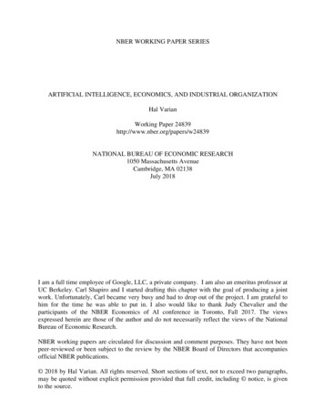
Transcription
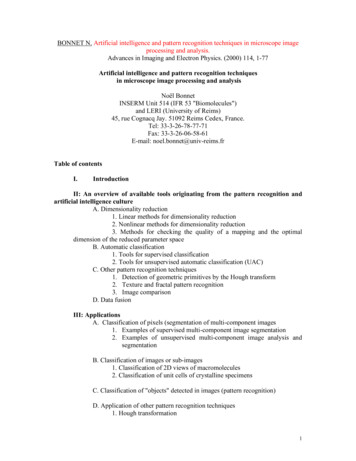
BONNET N. Artificial intelligence and pattern recognition techniques in microscope imageprocessing and analysis.Advances in Imaging and Electron Physics. (2000) 114, 1-77Artificial intelligence and pattern recognition techniquesin microscope image processing and analysisNoël BonnetINSERM Unit 514 (IFR 53 "Biomolecules")and LERI (University of Reims)45, rue Cognacq Jay. 51092 Reims Cedex, France.Tel: 33-3-26-78-77-71Fax: 33-3-26-06-58-61E-mail: noel.bonnet@univ-reims.frTable of contentsI.IntroductionII: An overview of available tools originating from the pattern recognition andartificial intelligence cultureA. Dimensionality reduction1. Linear methods for dimensionality reduction2. Nonlinear methods for dimensionality reduction3. Methods for checking the quality of a mapping and the optimaldimension of the reduced parameter spaceB. Automatic classification1. Tools for supervised classification2. Tools for unsupervised automatic classification (UAC)C. Other pattern recognition techniques1. Detection of geometric primitives by the Hough transform2. Texture and fractal pattern recognition3. Image comparisonD. Data fusionIII: ApplicationsA. Classification of pixels (segmentation of multi-component images1. Examples of supervised multi-component image segmentation2. Examples of unsupervised multi-component image analysis andsegmentationB. Classification of images or sub-images1. Classification of 2D views of macromolecules2. Classification of unit cells of crystalline specimensC. Classification of "objects" detected in images (pattern recognition)D. Application of other pattern recognition techniques1. Hough transformation1
2. Fractal analysis3. Image comparison4. Hologram reconstructionE. Data fusionIV. ConclusionAcknowledgementsReferences2
I : IntroductionImage processing and analysis play an important and increasing role in microscopeimaging. The tools used for this purpose originate from different disciplines. Many of themare the extensions of tools developed in the context of one-dimensional signal processing toimage analysis. The signal theory furnished most of the techniques related to the filteringapproaches, where the frequency content of the image is modified to suit a chosen purpose.Image processing is, in general, linear in this context. On the other hand, many nonlinear toolshave also been suggested and widely used. The mathematical morphology approach, forinstance, is often used for image processing, using gray level mathematical morphology, aswell as for image analysis, using binary mathematical morphology. These two classes ofapproaches, although originating from two different sources, have interestingly been unifiedrecently within the theory of image algebra (Ritter, 1990; Davidson, 1993; Hawkes, 1993,1995).In this article, I adopt another point of view. I try to investigate the role already played(or that could be played) by tools originating from the field of artificial intelligence. Ofcourse, it could be argued that the whole activity of digital image processing represents theapplication of artificial intelligence to imaging, in contrast with image decoding by the humanbrain. However, I will maintain throughout this paper that artificial intelligence is somethingspecific and provides, when applied to images, a group of methods somewhat different fromthose mentioned above. I would say that they have a different flavor. People who feelcomfortable in working with tools originating from the signal processing culture or themathematical morphology culture do not generally feel comfortable with methods originatingfrom the artificial intelligence culture, and vice versa. The same is true for techniques inspiredby the pattern recognition activity.In addition, I will also try to evaluate whether or not tools originating from patternrecognition and artificial intelligence have diffused within the community of microscopists. Ifnot, it seems useful to ask the question whether the future application of such methods couldbring something new to microscope image processing and if some unsolved problems couldtake advantage of this introduction.The remaining paper is divided into two parts. The first part (section II) consists of a(classified) overview of methods available for image processing and analysis in theframework of pattern recognition and artificial intelligence. Although I do not pretend to havediscovered something really new, I will try to give a personal presentation and classificationof the different tools already available. Then, the second part (section III) will be devoted tothe application of the methods described in the first part to problems encountered inmicroscope image processing. This second part will be concerned with applications whichhave already started as well as potential applications.II: An overview of available tools originating from thepattern recognition and artificial intelligence cultureThe aim of Artificial Intelligence (AI) is to stimulate the developments of computeralgorithms able to perform the same tasks that are carried out by human intelligence. Somefields of application of AI are automatic problem solving, methods for knowledgerepresentation and knowledge engineering, for machine vision and pattern recognition, forartificial learning, automatic programming, the theory of games, etc (Winston, 1977).Of course, the limits of AI are not perfectly well defined, and are still changing withtime. AI techniques are not completely disconnected from other, simply computational,techniques, such as data analysis, for instance. As a consequence, the list of topics included in3
this review is somewhat arbitrary. I chose to include the following ones: dimensionalityreduction, supervised and unsupervised automatic classification, neural networks, data fusion,expert systems, fuzzy logic, image understanding, object recognition, learning, imagecomparison, texture and fractals. On the other hand, some topics have not been included,although they have some relationships with artificial intelligence and pattern recognition. It isthe case, for instance, of methods related to the information theory, to experimental design, tomicroscope automation and to multi-agents system.The topics I have chosen are not independent of each other and the order of theirpresentation is thus rather arbitrary. Some of them will be discussed in the course of thepresentation of the different methods. The rest will be discussed at the end of this section.For each of the topics mentioned above, my aim is not to cover the whole subject (acomplete book would not be sufficient), but to give the unfamiliar reader the flavor of thesubject, that is to say, to expose it qualitatively. Equations and algorithms will be given onlywhen I feel they can help to explain the method. Otherwise, references will be given toliterature where the interested reader can find the necessary formulas.A. Dimensionality reductionThe objects we have to deal with in digital imaging may be very diverse: they can bepixels (as in image segmentation, for instance), complete images (as in image classification)or parts (regions) of images. In any case, an object is characterized by a given number ofattributes. The number of these attributes may also be very diverse, ranging from one (thegray level of a pixel, for instance) to a huge number (4096 for a 64x64 pixels image, forinstance). This number of attributes represents the original (or apparent) dimensionality of theproblem at hand, that I will call D. Note that this value is sometimes imposed by experimentalconsiderations (how many features are collected for the object of interest), but is alsosometimes fixed by the user, in the case the attributes are computed after the image isrecorded and the objects extracted; think of the description of the boundary of a particle, forinstance. Saying that a pattern recognition problem is of dimensionality D means that thepatterns (or objects) are described by D attributes, or features. It also means that we have todeal with objects represented in a D-dimensional space.A “common sense” idea is that working with spaces of high dimensionality is easierbecause patterns are better described and it is thus easier to recognize them and todifferentiate them. However, this is not necessarily true because working in a space with highdimensionality also has some drawbacks. First, one cannot see the position of objects in aspace of dimension greater than 3. Second, the parameter space (or feature space) is then verysparse, i.e. the density of objects in that kind of space is low. Third, as the dimension of thefeature space increases, the object description becomes necessarily redundant. Fourth, theefficiency of classifiers starts to decrease when the dimensionality of the space is higher thanan optimum (this fact is called the curse of dimensionality). For these different reasons whichare interrelated, reducing the dimensionality of the problem is often a requisite. This meansmapping the original (or apparent) parameter space onto a space with a lower dimension(ℜD ℜD’; D’ D). Of course, this has to be done without losing information, which meansremoving redundancy and noise as much as possible, without discarding useful information.For this, it would be fine if the intrinsic dimensionality of the problem (that is, the sizeof the subspace which contains the data, which differs from the apparent dimensionality)could be estimated. Since very few tools are available (at the present time) for estimating theintrinsic dimensionality reliably, I will consider that mapping is performed using trial-anderror methods and the correct mapping (corresponding to the true dimensionality) is selectedfrom the outcome of these trials.4
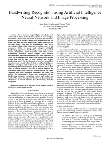
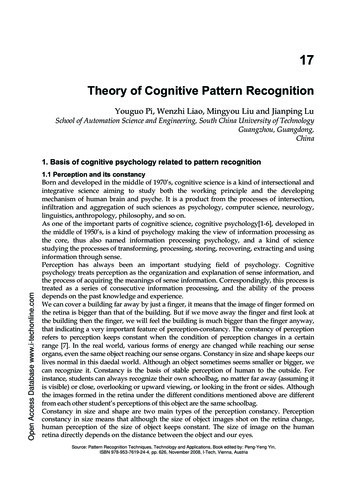
Many approaches have been investigated for performing this mapping onto a subspace(Becker and Plumbey, 1996). Some of them consist of feature (or attribute) selection. Othersconsist in computing a reduced set of features out of the original ones. Feature selection is ingeneral very application-dependent. As a simple example, just consider the characterization ofthe shape of an object. Instead of keeping as descriptors all the contour points, it would bebetter to retain only the points with high curvature, because it is well known that they containmore significant information than points of low curvature. They are also stable in the scalespace configuration.I will concentrate on feature reduction. Some of the methods for doing this are linear,while others are not.1. Linear methods for dimensionality reductionMost of the methods used so far for performing dimensionality reduction belong to thecategory of Multivariate Statistical Analysis (MSA) (Lebart et al., 1984). They have beenused a lot in electron microscopy and microanalysis, after their introduction at the beginningof the eighties, by Frank and Van Heel (Van Heel and Frank, 1980, 1981; Frank and VanHeel, 1982) for biological applications and by Burge et al. (1982) for applications in materialsciences. The overall principle of MSA consists in finding principal directions in the featurespace and to map the original data set onto these new axes of representation. The principaldirections are such that a certain measure of information is maximized. According to thechosen measure of information (variance, correlation, etc.), several variants of MSA areobtained such as Principal Components Analysis (PCA), Karhunen Loëve Analysis (KLA),Correspondence Analysis (CA). In addition, the different directions of the new subspace areorthogonal.Since MSA has become a traditional tool, I will not develop its description in thiscontext; see references above and Trebbia and Bonnet (1990) for applications inmicroanalysis.At this stage, I would just like to illustrate the possibilities of MSA through a singleexample. This example, which I will use in different places throughout this part of the paperfor the purpose of illustrating the methods, concerns the classification of images contained ina set; see section III.B for real applications to the classification of macromolecule images. Theimage set is constituted of thirty simulated images of a “face”. These images form threeclasses with unequal populations, with five images in class 1, ten images in class 2 and fifteenimages in class 3. They differ by the gray levels of the “mouth”, the “nose” and the “eyes”.Some within-class variability was also introduced, and noise was added. The classes weremade rather different, so that the problem at hand can be considered as much easier to solvethan real applications. Nine (out of thirty) images are reproduced in Figure 1. Some of theresults of MSA (more precisely, Correspondence Analysis) are displayed in Figure 2. Figure2a displays the first three eigenimages, i.e. the basic sources of information which composethe data set. These factors represent 30%, 9% and 6% of the total variance, respectively.Figure 2b represents the scores of the thirty original images onto the first two factorial axes.Together, these two representations can be used to interpret the original data set: eigen-imageshelp to explain the sources of information (i.e. of variability) in the data set (in this case,“nose”, “mouth” and “eyes”) and the scores allow us to see which objects are similar ordissimilar. In this case, the grouping into three classes (and their respective populations) ismade evident through the scores on two factorial axes only. Of course, the situation is notalways as simple because of more factorial axes containing information, overlapping clusters,etc. But linear mapping by MSA is always useful.One advantage of linearity is that once sources of information (i.e. eigenvectors of thevariance-covariance matrix decomposition) are identified, it is possible to discard5
uninteresting ones (representing essentially noise, for instance) and to reconstitute a cleaneddata set (Bretaudière and Frank, 1988).I would just like to comment on the fact that getting orthogonal directions is notnecessarily a good thing, because sources of information are not necessarily (and often arenot) orthogonal. Thus, if one wants to quantify the true sources of information in a data set,one has to move from orthogonal, abstract, analysis to oblique analysis (Malinowski andHowery, 1980). Although these things are starting to be considered seriously in spectroscopy(Bonnet et al., 1999a), the same is not true in microscope imaging except as reported by Kahnand collaborators, see section III.A, who introduced the method that was developed by theirgroup for medical nuclear imaging in confocal microscopy studies.2. Nonlinear methods for dimensionality reductionMany trials to perform dimensionality reduction more efficiently than with MSA havebeen attempted. Getting a better result requires the introduction of nonlinearity. In thissection, I will describe heuristics and methods based on the minimization of a distortionmeasure, as well as neural-networks based approaches.a. Heuristics:The idea here is to map a D-dimensional data set onto a 2-dimensional parameterspace. This reduction to two dimensions is very useful because the whole data set can thus bevisualized easily through the scatterplot technique. One way to map a D-space onto a 2-spaceis to “look” at the data set from two observation positions and to code what is “seen” by thetwo observers. In Bonnet et al. (1995b), we described a method where observers are placed atcorners of the D-dimensional hyperspace and the Euclidean distance from an observer anddata points is coded as the information “seen” by the observer. Then, the coded information“seen” by two such observers is used to build a scatterplot.From this type of method, one can get an idea of the maximal number of clusterspresent in the data set. But no objective criterion was devised to select the best pairs ofobservers, i.e. those which preserve the information maximally. More recently, we suggesteda method for improving this technique (Bonnet et al., in preparation), in the sense thatobservers are automatically moved around the hyperspace defined by the data set in such away that a quality criterion is optimized. This criterion can be either the type of criteriondefined in the next section or the entropy of the scatterplot, for instance.b. Methods based on the minimization of a distortion measureConsidering that, in a pattern recognition context, distances between objects constituteone of the main sources of information in a data set, the sum of the differences between interobject distances (before and after nonlinear mapping) can be used as a distortion measure.This criterion can thus be retained to define a strategy for minimum distortion mapping. Thisstrategy has been suggested by psychologists a long time ago (Kruskal, 1964; Shepard, 1966;Sammon, 1969).Several variants of such criteria have been suggested. Kruskal introduced thefollowing criterion in his Multidimensional Scaling (MDS) method:EMDS (Dij dij )2i(1)j iwhere Dij is the distance between objects i and j in the original feature space and dij is thedistance between the same objects in the reduced space.Sammon (1969) introduced the relative criterion instead:6
ES ij i( Dij d ij ) 2Dij(2)Once a criterion is chosen, the way to arrive at the minimum, thus performing optimalmapping, is to move the objects in the output space (i.e. changing their coordinates x )according to some variant of the steepest gradient method, for instance. As an example, theminimization of Sammon’s criterion can be obtained according to the Newton’s method as:AB D d ij E ( xil x jl )where A S ij xilj Dij .d ij xt 1 xt α .B (3)(xil xjl )2 1 Dij dij 2ES1 Dd j D .d ij ij d d xil2 ij ij ijij and t is the iteration index.It should be stressed that the algorithmic complexity of these minimization processesis very high, since N2 distances (where N is the number of objects) have to be computed eachtime an object is moved in the output space. Thus, faster procedures have to be explored whenthe data set is composed of many objects. Some examples of improving the speed of suchmapping procedures are:- selecting (randomly or not) a subset of the data set, performing the mapping ofthese prototypes, and calculating the projections of the other objects afterconvergence, according to their original position with respect to the prototypes- modifying the mapping algorithm in such a way that all objects (instead of onlyone) are moved in each iteration of the minimization process (Demartines, 1994).Other methodsBesides the distortion minimization methods and the heuristic approaches describedabove, several artificial neural-networks approaches have also been suggested. The SelfOrganizing Mapping (SOM) method (Kohonen) and the Auto-Associative Neural Network(AANN) method are most commonly used in this context.c. SOMSelf-organizing maps are a kind of artificial neural network which are supposed toreproduce some parts of the human visual or olfactive systems, where input signals are selforganized in some regions of the brain. The algorithm works as follows (Kohonen, 1989):- a grid of reduced dimension (two in most cases, sometimes one or three) is created,with a given topology of interconnected neurons (the neurons are the nodes of thegrid and are connected to their neighbors, see Figure 3),- each neuron is associated with a D-dimensional feature vector, or prototype, orcode vector (of the same dimension as the input data),- when an input vector xk is presented to the network, the closest neuron (the onewhose associated feature vector is at the smallest Euclidean distance) is searchedand found: it is called the winner,- the winner and its neighbors are updated in such a way that the associated featurevectors υi come closer to the input:υi,t 1 υi,t αt . (xk - υi,t)i ηt(4)7
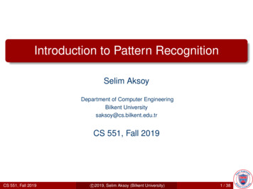
where αt is a coefficient decreasing with the iteration index t, ηt is a neighborhood,also decreasing in size with t.This process constitutes a kind of unsupervised learning called competitive learning. It resultsin a nonlinear mapping of a D-dimensional data set onto a D’-dimensional space: objects cannow be described by the coordinates of the winner on the map. It possesses the property oftopological preservation: similar objects are mapped either to the same neuron or to close-byneurons.When the mapping is performed, several tools can be used for visualizing andinterpreting the results:- the map can be displayed with indicators proportional to the number of objectsmapped per neuron,- the average Euclidean distance between a neuron and its four or eight neighborscan be displayed, to identify clusters of similar neurons,- the maximum distance can be used instead (Kraaijveld et al., 1995)An illustration of self-organizing mapping, performed on the thirty simulated imagesdescribed above, is given in Figure 4.SOM has many attractive properties but also some drawbacks which will be discussedin a later section.Ideally, the dimensionality (1, 2, 3, ) of the grid should be chosen according to theintrinsic dimensionality of the data set, but this is often not the way it is done. Instead, sometricks are used, such as hierarchical SOM (Bhandarkar et al., 1997) or nonlinear SOM (Zhenget al., 1997), for instance.d. AANN:The aim of auto-associative neural-networks is to find a representation of a data set ina space of low dimension, without losing much information. The idea is to check whether theoriginal data set can be reconstituted once it has been mapped (Baldi and Hornik, 1989;Kramer, 1991).The architecture of the network is displayed in Figure 5. The network is composed offive layers. The first and the fifth layers (input and output layers) are identical, and composedof D neurons, where D is the number of components of the feature vector. The third layer(called the bottleneck layer) is composed of D’ neurons, where D’ is the number ofcomponents anticipated for the reduced space. The second and fourth layers (called the codingand decoding layers) contain a number of neurons intermediate between D and D’. Their aimis to compress (and decompress) the information before (after) the final mapping. It has beenshown that their presence is necessary. Due to the shape of the network, it is sometimes calledthe Diabolo network.The principle of the artificial neural network is the following: when an input ispresented, the information is carried through the whole network (according to the weight ofeach neuron) until it reaches the output layer. There, the output data should be as close to theinput data as possible. Since this is not the case at the beginning of the training phase, theerror (squared difference between input and output data) is back-propagated from the outputlayer to the input layer. Error back-propagation will be described a little bit more precisely inthe section devoted to multi-layer feed-forward neural networks. Thus, the neuron weights areupdated in such a way that the output data more closely resembles the input data. Afterconvergence, the weights of the neurons are such that a correct mapping of the original (Ddimensional) data set can be performed on the bottleneck layer (D’-dimensional). Of course,this can be done without too much loss of information only if the chosen dimension D’ iscompatible with the intrinsic dimensionality of the data set.8
e. Other dimensionality reduction approachesIn the previous paragraphs, the dimensionality reduction problem was approached byabstract mathematical techniques. When the "objects" considered have specific properties, itis possible to envisage (and even to recommend) how to exploit these properties forperforming dimensionality reduction.One example of this approach consists in replacing images of centro-symmetricparticles by their rotational power spectrum (Crowther and Amos, 1971): the image is splitinto angular sectors, the summed signal intensity within the sectors is then Fouriertransformed to give a one-dimensional signal containing the useful information related to therotational symmetry of the particles.3. Methods for checking the quality of a mapping and the optimal dimension ofthe reduced parameter spaceChecking the quality of a mapping for selecting one mapping method over others isnot an easy task and depends on the criterion chosen to evaluate the quality. Suppose, forinstance, that the mapping is performed through an iterative method aimed at minimizing adistortion measure e.g. as MDS or Sammon’s mappings do. If the quality criterion chosen isthe same distortion measure, this method will be found to be good, but the same result maynot be true if other quality criteria are chosen. Thus, one has sometimes to evaluate the qualityof the mapping through the evaluation of a subsidiary task, such as classification of knownobjects after dimensionality reduction (see for instance De Baker et al. 1998).Checking the quality of the mapping may also be a way to estimate the intrinsic (ortrue) dimensionality of the data set, that is to say the optimum reduced dimension (D’) for themapping, or in other words the smallest dimension of the reduced space for which most of theoriginal information is preserved.One useful tool for doing this (and checking the different results visually) is to drawthe scatterplot relating the new inter-distances (dij) to the original ones (Dij). While mostinformation is preserved, the scatterplot display remains concentrated along the first diagonal(dij Dij i j). On the other hand, when some information is lost because of excessivedimensionality reduction, the scatterplot is no longer concentrated along the first diagonal,and distortion concerning either small distances or large distances (or both) becomesapparent.Besides visual assessment, the distortion can be quantified through several descriptorsof the scatterplot, such as:2(5)- contrast: C ( D' ) (Dij d ij ) . p (Dij , d ij )ij iij i[]- entropy: E ( D' ) p (Dij , d ij ). log p (Dij , d ij )(6)where p(Dij,dij) is the probability that the original and post-mapping distances between objectsi and j take the values Dij and dij, respectively. Plotting C(D’) or E(D’) as a function of thereduced dimensionality D’ allows us to check the behavior of the data mapping. A rapidincrease in C or E when D’ decreases is often the sign of an excessive reduction in thedimensionality of the reduced space. The optimality of the mapping can be estimated as anextremum of the derivative of one of these criteria.Figure 6 illustrates the process described above. The data set composed of the thirtysimulated images was mapped onto spaces of dimension 4, 3, 2 and 1, according to Sammon’smapping. The scatterplots relating the distances in the reduced space to the original distancesare displayed in Figure 6a. One can see that a large change occurs for D’ 1, indicating that9
this is too large a dimensionality reduction. This visual impression is confirmed by Figure 6b,which displays the behavior of the Sammon criterion for D’ varying from 4 to 1.These tools may be used whatever the method used for mapping including MSA andneural networks.According to the results obtained by De Baker et al. (1998), nonlinear methodsprovide better results than linear methods for the purpose of dimensionality reduction.Event coveringAnother topic connected to the discussion above concerns the interpretation of thedifferent axes of representation after performing linear or nonlinear mapping. Thisinterpretation of axes in terms of sources of information is not always an easy task. Harauzand Chiu (1991, 1993) suggested the use of the event-covering method, based on hierarchicalmaximum entropy discretization of the reduced feature space. They showed that thisprobabilistic inference method can be used to choose the best components upon which to basea clustering, or to appropriately weight the factorial coordinates to under-emphasizeredundant ones.B. Automatic classificationEven when they are not perceived as such, many problems in intelligent imageprocessing are, in fact, classification problems. Image segmentation, for instance, be itunivariate or multivariate, consists in the classification of pixels, either into different classesrepresenting different regions, or into boundary/non-boundary pixels. Automatic classificationis one of the most important problems in artificial intelligence and covers many of the othertopics in this category such as expert systems, fuzzy logic and some neural networks, forinstance.Traditionally, automatic classification has been subdivided into two very differentclasses of activity, namely supervised classification and unsupervised classification. Theformer is done under the control of a supervisor or a trainer. The supervisor is an expert in thefield of application who furnishes a training set, that is to say a set of known prototypes foreach class, from which the system must be able to learn how to move from the parameter (orfeature) space to the decision space. Once the training phase is completed (which cangenerally be done if and only if the training set is consistent and complete), the sameprocedure can be followed for unknown objects and a decision can be made to classify theminto one of the existing classes or into a reject class.In contrast, unsupervised automatic classification (also called clustering) does notmake use of a training set. The classification is attempted on the basis of the data set itself,assuming that clusters of similar objects exist (principle of internal cohesion), and thatboundaries can be found which enclose clusters of similar objects and disclose clusters ofdissimilar objects (principle of external isolation).1. Tools for supervised classificationTools available for performing supervised automatic classification are numerous. Theyinclude interactive tools and automatic tools. One method in the first group is InteractiveCorrelation Part
pattern recognition and artificial intelligence culture The aim of Artificial Intelligence (AI) is to stimulate the developments of computer algorithms able to perform the same tasks that are carried out by human intelligence. Some fields of application o