Transcription
Lecture Notes onSolid State PhysicsKevin Zhoukzhou7@gmail.comThese notes comprise an undergraduate-level introduction to solid state physics. Results fromundergraduate quantum mechanics are used freely, but the language of second quantization is not.The primary sources were: Kittel, Introduction to Solid State Physics. The standard undergraduate-level introduction tosolid state physics, with consistently good quality. Ashcroft and Mermin, Solid State Physics. The standard graduate-level introduction to solidstate physics. Relatively dry and difficult to read. Covers essentially the same conceptualmaterial as Kittel, with more detail on specific properties of solids and experimental techniques. Simon, The Oxford Solid State Basics. A new book that covers most of the material in Kittel.More modern than any other solid state book at this level, with clear, clean explanationsthroughout. Also has the huge advantage of using Dirac notation over wavefunctions, whichshortens and clarifies almost every equation. Has well-written, helpful problems. David Tong’s lecture notes on Applications of Quantum Mechanics. Covers much of the materialof Simon’s book, also in clear modern notation, with a conversational tone. Also contains niceasides on topics like graphene and the Peierls instability. Annett, Superconductivity, Superfluids, and Condensates. A very clear first book on thesephenomena, both describing their basic phenomenology and connecting it to microscopic theory.Uses many body theory, but with a very light touch. The Feynman Lectures on Physics, volume 2. About ten chapters cover properties of materials.Entertaining bedtime reading, though a number of statements are out of date.The most recent version is here; please report any errors found to kzhou7@gmail.com.
2 ContentsContents1 Free Electron Models1.1 Introduction . . . . . . . . . . . . . . . . . . . . . . . . . . . . . . . . . . . . . . . . .1.2 Drude Theory . . . . . . . . . . . . . . . . . . . . . . . . . . . . . . . . . . . . . . . .1.3 Sommerfeld Theory . . . . . . . . . . . . . . . . . . . . . . . . . . . . . . . . . . . . .33482 Crystal Structure2.1 Bloch’s Theorem . . .2.2 Bravais Lattices . . . .2.3 The Reciprocal Lattice2.4 X-ray Diffraction . . .10101317193 Band Structure3.1 Bloch Electrons . . . .3.2 Tight Binding . . . . .3.3 Nearly Free Electrons3.4 Phonons . . . . . . . .3.5 Band Degeneracy . . .2323252830334 Applications of Band Structure4.1 Electrical Conduction . . . . . . . . . . . . . . . . . . . . . . . . . . . . . . . . . . .4.2 Magnetic Fields . . . . . . . . . . . . . . . . . . . . . . . . . . . . . . . . . . . . . . .4.3 Semiconductor Devices . . . . . . . . . . . . . . . . . . . . . . . . . . . . . . . . . . .373741435 Magnetism485.1 Paramagnetism and Diamagnetism . . . . . . . . . . . . . . . . . . . . . . . . . . . . 485.2 Ferromagnetism . . . . . . . . . . . . . . . . . . . . . . . . . . . . . . . . . . . . . . . 526 Linear Response6.1 Response Functions . . . . . . . . . . . . . . . . . . . . . . . . . . . . . . . . . . . . .6.2 Kramers–Kronig . . . . . . . . . . . . . . . . . . . . . . . . . . . . . . . . . . . . . .6.3 The Kubo Formula . . . . . . . . . . . . . . . . . . . . . . . . . . . . . . . . . . . . .58585963
3 1. Free Electron Models1Free Electron Models1.1IntroductionIn these notes, we investigate properties of solids. We would like to ask: What is the global ground state of the atoms? Is it a periodic crystal, and if so, what is thecrystal structure? Does it agree with the results of X-ray diffraction? Given the crystal structure, what are the properties of the solid? For example, can we calculatethe thermal and electrical conductivity, color, hardness, magnetic susceptibility, resistivity, etc.? Resistivity is an especially interesting quantity, since it can range over 30 orders of magnitudebetween metals and insulators. Can we explain this dramatic difference in behavior?In principle, we have a “theory of everything” for solids, given by the HamiltonianH X 2X 2X Zα e 2XX Zα Zβ e2e2 2j 2α 2m2Mα ri Rα ri rk Rα Rβ αjj,αj kα βwhere capital letters/Greek indices denote lattice ions and lowercase letters/Latin indices denoteelectrons. However, in a solid, with O(1023 ) nuclei and electrons, solving this Hamiltonian exactly isinfeasible. In fact, the situation is more like QCD than perturbative QFT. Couplings are generallystrong, and perturbation theory can fail. Instead, we must use better approximations. First, we can use adiabatic approximations. Since the electrons are much less massive than theions, the ions move very slowly, and we may treat their effect on the electrons adiabatically.This yields the Born-Oppenheimer approximation. Second, we may use independent particle approximations. By neglecting electron-electron interactions, we may approximate the behavior of the full N -body interacting system by consideringthe behavior of a single electron. Third, we may use field theory methods. Suppose we can write the Hamiltonian in the formXH 0 E0 0k αk† αk f (. . . , αk , . . . , αk† 0 , . . .).kThen the low-lying degrees of freedom behave like independent harmonic oscillators. If f issmall, we can treat it perturbatively. This approach is useful because many properties of solidsonly depend on the low-lying excitations. There will generally be two kinds of excitations: quasiparticles, or ‘dressed’ particles, thatresemble a single free particle, and ‘collective excitations’ which are due to many particles.First, we’ll consider very basic ‘free electron’ models, which completely neglect interactions ofthe electrons with the lattice ions; such an approach can only be a good approximation for metals.Next, we reintroduce the lattice ions, leading to a discussion of band structure. Much later, we’llreintroduce interactions between electrons, leading to many body/field theory methods. We’llsee that the structure of the Fermi sea tends to make interactions unimportant in some contexts,retroactively justifying the neglect of interactions.
4 1. Free Electron Models1.2Drude TheoryThe Drude theory of metals, introduced in 1900, models a metal as a classical gas of electrons,assumed to be the valence electrons of the atoms used to form the metal. We assume the electrons don’t interact with each other at all, the ‘independent electron approximation’. However, we will allow collisions with the lattice ions. We take the ‘free electronapproximation’, assuming that in between collisions, the electrons are completely free, with theexception that the ions act as a ‘wall’ preventing the electrons from leaving the metal. We assume that collisions instantaneously randomize the velocity of an electron, so that itsmean final velocity is zero, and that they occur in a time dt with probability dt/τ , where τ isthe relaxation time. If we wanted to treat the collisions more carefully, we could choose the speed distribution aftera collision so that the electrons thermalize appropriately over time. It is difficult to calculate the collision rate τ 1 . There are many contributions, includingscattering off impurities, phonons, and other electrons. One might estimate τ 1/nσv whereσ is the cross section, but the cross section is infinite for the Coulomb fields of electron-electronscattering; the collisions simply aren’t sharp as assumed by Drude theory. Instead, we take τas a phenomenological parameter.Next, we consider the effects of static fields. Suppose the electrons experience an external force F and have average momentum hpi. Thendhpihpi Fdtτwhere the first term accounts for collisions. For simplicity we drop the brackets below. The average current density is given byj nep.mFor a static electric field, we thus havep eEτ,j σE,σDC ne2 τ.m Next, we consider the Hall effect. Suppose we apply an electric field Ex and a transversemagnetic field Bz . Then the Lorentz force should deflect electrons in the y direction, causing abuildup of charge on the side of the metal and creating a transverse field Ey . More formally, let E ρj where ρ is the resistivity tensor. Again working in the steady state,and restricting to a two-dimensional sample in the xy plane, 1mE j B 2 jnene τ
51. Free Electron Modelsfrom which we read off ρ,ρ m/ne2 τ B/neB/nem/ne2 τ 1σDC 1 ωB τωB τ1 where ωB eB/m is the cyclotron frequency. Note that ρ had to be antisymmetric by rotationalinvariance. We conventionally report the Hall coefficientRH ρxy1 .BneThis is especially useful because τ , which depends on messy details, cancels out. Another usefulfact is that in practice, we measure transverse resistances, butRxy VyLEyEy ρxyIxLJxJxso this is equivalent to a measurement of RH . Note this is particular to two-dimensional samples. Finally, it is sometimes useful to know the conductivity, σDC1 ωB Tσ .2 τ2 ω τ11 ωBB Strikingly, the Hall coefficient depends on the sign of the charge carriers, so it can be used toshow that charge carriers have negative charge. But even more strikingly, this fails! The Hallcoefficient is measured to have the opposite of the expected sign in some common materials,such as Be and Mg. It is also measured to be anisotropic. These results will be explained bycrystal and band structure below. In practice, the Hall effect can be used in reverse to detect magnetic fields, using a Hall sensor.To make the measured voltages large, Hall sensors use materials with a low density of electrons,such as semiconductors. Drude theory works very well for semiconductors.Next, we consider AC fields. We consider an electric field with frequency ω, sodpp eE0 e iωt .dtτThe momentum is also sinusoidal, and we find the frequency-dependent conductivityσ(ω) σDC,1 iωτj(ω) σ(ω)E(ω).Note that this is only sensible if λ where is the mean free path, since we’ve neglected thespatial variation of the field.
61. Free Electron Models It is useful to consider the limit τ . Naively we would havelim σ(ω) τ ne2iωmbut the real part requires a bit more care. We haveRe σ(ω) τne2m 1 ω2τ 2which is a Lorentzian with width 1/τ and total area πne2 /m. Hence we havelim σ(ω) τ πns e2ne2δ(ω) .meiωmThis indicates that j and E are 90 out of phase except for DC fields, where they are in phase. Now suppose we pass an electromagnetic wave through the material. It can be shown that thedielectric constant is related to the conductivity by (ω) 1 4πiσ(ω).ωAt low frequencies, the imaginary part of yields an exponential damping, corresponding toabsorption of light. For high frequencies, we have (ω) 1 ωp2,ω2ωp2 4πne2mwhere ωp is called the plasma frequency, and is notably independent of τ . In this regime, themetal is transparent. For intermediate frequencies, has a negative real part, which meansthere are only evanescent waves, so the metal is reflective. In the more realistic Lorentz oscillator model, we account for the lattice ions by putting everycharge carrier on a spring, and replace the collisions with a damping term. At low frequencies,light is transmitted, because the spring suppresses the charges’ response. At the resonantfrequency ω0 of the spring, we get strong absorption, while for higher frequencies we find thesame features as above, since the spring won’t matter. We can also consider an AC electric field in the presence of a transverse DC magnetic field. Onefinds that the conductivity sharply peaks when ω eB/m, diverging in the limit τ 0. Thisis called the cyclotron resonance; a large current is built up by resonance with the cyclotronfrequency. The cyclotron resonance may be used to measure m, and it is generally found thatm 6 me , another consequence of band structure.Finally, we turn to the thermal conductivity. The thermal conductivity is defined asjq κ Twhere jq is the heat current. We may calculate it crudely for gases using kinetic theory.
7 1. Free Electron Models In one dimension, suppose that particles have a typical velocity v and move a distance τ beforebeing scattered. If the energy per particle is E(T (x)), thenjq nvdE dT(E(T (x vτ )) E(T (x vτ ))) nv 2 τ.2dT dxHere dE/dT cv is the heat capacity per particle, soκ hv 2 incv τ3where we divided by three to account for the three spatial dimensions. Next, using the standard results13mhv 2 i kB T,223cv kB T2we conclude that2T3 nτ kB.2 mThis still depends on the unknown parameter τ , but it cancels out in the ratioκ L 2κ3 kB σT2 e2called the Lorenz number. The Wiedemann-Franz law states that L is approximately constant and temperature-independentacross many metals. In the Drude model, the entire analysis above carries over for metals without any change, so it explains the law. The derivation above is off by constant factors. More seriously, it doesn’t account for the factthat electrons are fermions, which makes cv much smaller than expected and v much higherthan expected. Luckily, both of these errors mostly cancel. To see this more sharply, we can consider the thermoelectric effect, which is the fact that anelectrical current also transports heat,jq Πj.To understand this classically, note that in regions of lower temperature, the typical velocitiesare lower; in the Drude model this appears in the speed distribution after scattering. Henceelectrons pile up in regions of lower temperature, producing a gradient of electric potentialalongside a gradient of temperature. On the quantum level, the change in temperature insteadchanges the Fermi level, providing the imbalance of electrons. Various aspects of the thermoelectric effect are called the Peltier, Seebeck, and Thomson effects.They may be used for refrigeration devices. Since both jq and j are proportional to v, it cancels to yieldΠ cv TkB T .3e2eHowever, this prediction is off by a factor of 100, and has the wrong sign in some metals.
81. Free Electron Models1.3Sommerfeld TheorySommerfeld theory fixes some of the problems of Drude theory by replacing its Maxwell-Boltzmanndistribution with a Fermi-Dirac distribution. Considering a box of volume V with N electrons at zero temperature, we haveZ kFN 2Vd̄kwhere kF is the Fermi wavevector and the 2 accounts for the two spin states of the electron.For convenience we define the Fermi energy, temperature, momentum, and velocity byEF 2 kF2,2mTF EF,kBpF kF ,vF kF.m Performing the integral, we findkF (3π 2 n)1/3 .Numerically, for a typical metal, this impliesEF 10 eV,TF 105 K,vF c.100We see T TF is always true for metals, since they melt at a far lower temperature. It is also useful to define the density of states per unit volume,sm3/2 3nEg(E) 2 3 2E π 2EF3so that at finite temperatures,ZEEg(E) dE,V1 eβ(E µ)N VZdEg(E)1 eβ(E µ) Sommerfeld theory correctly predicts the electronic heat capacity, asE(T ) E(T 0) V g(EF )(kB T )2 ,C (N kB )T.TFHence the heat capacity is linear in the temperature, and smaller than the Drude result by afactor of T /TF . This may be measured at low temperatures, where the T 3 phonon contribution,which is typically much larger, is negligible. Using this result gives a reasonable result for Π. As for the Wiedemann-Franz law, we notethat hv 2 i is larger than in the Drude model by a factor of T /TF , which is why the Drude resultis approximately right. Sommerfeld theory also explains Pauli paramagnetism. Upon turning on a magnetic field, theFermi surfaces for spin up and spin down electrons shift in/out by energy µB B, which givesM g(EF )µ2B Bwhich is on the right order of magnitude, though again the sign is occasionally wrong.
91. Free Electron ModelsNext, we reflect on the successes and failures of these models. Some quantities calculated in the Drude model, such as RH , are on the right order of magnitudewithout Sommerfeld theory. At the simplest level, this is simply because they don’t dependdirectly on v. At a deeper level, it’s because they only require the equation of motiondpp Fdtτand in the context of Sommerfeld theory, we can take p to be the mean momentum of theentire Fermi sea! In this context, collisions are quite violent, since they require going from one end of the Fermisea to the other. In practice, such a process may be composed of many small scattering eventswhich move an electron around the Fermi sea. Neither Drude nor Sommerfeld theory cannot account for the number of conduction electrons,and hence cannot describe nonmetals. Similarly, they cannot account for the occasionallyopposite sign or modified mass of the charge carriers. Both are resolved by band structure. Unlike the predictions of free electron theory, the DC conductivity can be temperature-dependentand anisotropic. Moreover, the frequency dependence of the AC conductivity and hence theoptical spectrum is much more complicated than predicted. Thermodynamic properties such as the specific heat and equation of state are far off; the latticeions and electron-electron interactions are important here. Free electron theories cannot account for permanent magnetism, which crucially depends oninteractions. Moreover, they can’t explain why interactions can be ignored, since the Coulombinteraction energies are very large, on the order of the Fermi energy. The resolution is providedby Landau Fermi liquid theory.
10 2. Crystal Structure2Crystal Structure2.1Bloch’s TheoremWe now refine our theory of solids by accounting for the ionic lattice, which produces bands ofallowed and forbidden energy. For simplicity, we first show the physical effects in one dimension. Consider an electron in a periodic potential U of period a. The translation operator T (a) thuscommutes with the Hamiltonian, so they may be simultaneously diagonalized. The energyeigenfunctions hence take the formψ(x) uk (x)eikx ,uk (x a) uk (x).This result is called Bloch’s theorem, the eigenfunctions are called Bloch waves, and k is calledthe crystal momentum; note that it is only defined up to factors of 2π/a. Conventionally, we take the crystal momenta to lie in the first Brillouin zone [ π/a, π/a]. Thecrystal momenta are ambiguous by k k G, where the reciprocal lattice G contains elementsof the form 2πn/a. For a crystal of finite size, say with N lattice ions, the values of k are also quantized. Thereare N allowed values of k within the Brillouin zone. For each value of k, the function uk (x) obeys a Schrodinger equation with periodic boundaryconditions. Hence there are really multiple solutions, with quantized energy. In the limitN , the energy levels fill out “bands” of allowed and forbidden energy. Since the potential is periodic, its Fourier transform has support on the reciprocal latticeXU (x) UG eiGxGand since U (x) is real, UG U G . Plugging in the Fourier transformψ(x) XC(k)eikx ,kk 2πnLthe Schrodinger equation becomesXX k2X0C(k)eikx UG eiGx C(k 0 )eik x EC(k)eikx .2m0kkG,kSetting k 0 k G and setting the eikx Fourier coefficient to zero, 2 Xk E C(k) UG C(k G) 0.2mG This result gives us a better understanding of Bloch’s theorem. We see that scattering off thelattice can only exchange momenta in the reciprocal lattice. Therefore, every stationary statecan be built out of a linear combination of plane waves whose momenta differ by reciprocallattice vectors.
11 2. Crystal Structure The result above is not unfamiliar. An electron in an external field eiωt may absorb energyfrom the field in multiples of ω, so its energy is only conserved up to multiples of ω. Thelattice ions simply do the same with spatial variation. The crystal momentum is not the momentum of the electron. If an electron has crystalmomentum k, it has Fourier components at all k G. However, crystal momentum behavessomewhat like momentum. If a phonon carries crystal momentum q, then in an electron-phononinteraction k q is conserved, where again this quantity is only defined up to multiples of G.These multiples of G correspond to momentum being transferred to the lattice ions as a whole. Conceptually, momentum is the conserved quantity associated with spatial translations, whilecrystal momentum is the conserved quantity (up to G) associated with translation of excitationswithin a medium; this is more generally called pseudomomentum. In other words, the differenceis between translating the crystal and everything in it, and translating the phonon within thecrystal. A particle that interacts weakly with the crystal, such as an X-ray photon, has equal momentumand crystal momentum. However, a phonon with definite crystal momentum has precisely zeromomentum, because the only Fourier component with any momentum is the k 0 component.Hence when an X-ray photon scatters off a phonon, we can conclude momentum is transferred,but it is not given to the phonon but instead to the lattice as a whole. This remains true even if we account for momentum uncertainties. Suppose the phonon andscattered photon are both reasonably well-localized. Then the lattice configuration after thescattering is the superposition of wavepackets peaked near wavenumbers 0 and some k 6 0.However, since phonons generically have nontrivial dispersion, these wavepackets separatequickly, so it is not reasonable to attribute the momentum to the phonon. In the theory of liquids, one often works in an approximation where the dispersion is linear. Inthat case the wavepackets don’t separate, so one may attribute momentum to phonons.Note. To understand the appearance of band gaps, we can use the “nearly free electron model”.Starting from free electrons with a continuous spectrum ω k 2 /2m, turning on the potential splitsup the spectrum. Small band gaps appear because of the general phenomenon of level repulsion.More explicitly, suppose the potential is U (x) U0 cos(2πx/a), and consider the initially degeneratestates e ikπ/a . The new eigenstates are cosines and sines, and their probability accumulates eitherclose to, or far away from the atoms. These represent bonding and antibonding states.
12 2. Crystal StructureNote. To understand the appearance of bands, we can use the “tight binding model”. We begin withelectrons tightly bound to each lattice ion. Then we have discrete atomic energy levels. Allowingthe electrons to ‘hop’ between the atoms broadens these levels into small bands.Example. The Kronig-Penney model is a simple model of a solid, where we choose the potentialto be periodic and stepwise constant. More specifically, the ‘unit cell’ for the potential is(0 w x 0V (x) V00 x bWe assume that N , so we don’t have to worry about the periodic boundary conditions. Theperiod is a w b. The solutions in these two regions, assuming E V0 , are ψI (x) Aeiqx Be iqx , q(E) 2mEandψII (x) Ceβx De βx ,β(E) p2m(V0 E).The first two conditions are continuity of the wavefunction and its derivative,ψI (0) ψII (0),0ψI0 (0) ψII(0).We also have the same conditions at x w and x b, up to the Bloch phase factor eika ,ψII (b) eika ψI ( w),0ψII(b) eika ψI0 ( w).We find four linear equations for the coefficients A, B, C, and D. Since zero is a solution, the onlyway to get a nontrivial solution is if the determinant of the matrix of coefficients is zero. Evaluatingthis condition, we findβ 2 q2sinh βb sin qw cosh βb cos qw cos ka.2qβAs a further simplification, we may narrow the potentials to delta functions, taking b 0 whileV0 b is held constant; this givesPsin qa cos qa cos ka,qaP mV0 ba.As a function of qa, the left-hand side interpolates between sinc-like and cos-like. We only have asolution for k if the left-hand side is between 1 and 1. Therefore we find bands separated by gapsin q (and hence in E), as expected. For high q, the separation between the bands decreases, as theeffect of the potential becomes relatively weaker. This result is shown below.
13 2. Crystal Structure2.2Bravais LatticesWe now investigate 3D crystal structure in detail. A three-dimensional Bravais lattice is the set of all points of the formR n1 a1 n2 a2 n3 a3where the ai are linearly independent and the ni are integers. Alternatively, a Bravais lattice isa set of discrete points that looks exactly the same from every point, or a set of vectors closedunder addition. We say the ai are primitive lattice vectors and they generate/span the lattice. Note thatprimitive vectors are not unique; different equivalent sets of primitive vectors are related bymatrices A with integer entries and unit determinant. The coordination number of a Bravais lattice is the number of nearest neighbors of each point. A unit cell is a pattern that, when translated by a sublattice of a Bravais lattice, tiles the spaceperfectly. A primitive unit cell does the same when translated by any vector in the lattice.Primitive unit cells are far from unique, but all have the same volume, since they contain onelattice point each. One example of a primitive unit cell is the set{r x1 a1 x2 a2 x3 a3 0 xi 1}.However, note that this will often be less rotationally symmetric than the lattice as a whole. Anon-primitive ‘conventional’ unit cell is often picked to have the full symmetry of the lattice. The Wigner-Seitz cell about a lattice point is the set of points that are closer to that pointthan to any other point; it is a special case of a Voronoi cell. The cells are all identical by thedefinition of a Bravais lattices, so the Wigner-Seitz cell is indeed a primitive cell. Geometrically, the Wigner-Seitz cell may be constructed by drawing the planes of equidistantpoints between our chosen point and each other point in the lattice. It can be shown that theWigner-Seitz cell has the same symmetries as the lattice. For a real crystal, the Bravais lattice only reflects the underlying translational symmetry, butwe must also specify the positions of the atoms with respect to a unit cell; such a descriptionwith respect is called a basis.Example. The honeycomb lattice of graphene is not a Bravais lattice, since the lattice does notlook the same from any two neighboring points, but it is a Bravais lattice with a basis.
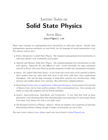
14 2. Crystal StructureThe underlying Bravais lattice is called a hexagonal, or triangular lattice. If the primitive vectorsare a1 and a2 , the basis is {(1/3)(a1 a2 ), (2/3)(a1 a2 )}.Example. A simple cubic lattice has primitive vectors x̂, ŷ, and ẑ. A body-centered cubic (bcc)lattice is the same, but adds an extra point in the center of each of the cubes.This is a Bravais lattice, since every point is surrounded by 8 neighbors in a cubic arrangement.One set of primitive vectors isa1 x̂,a2 ŷ,1a3 (x̂ ŷ ẑ).2Next, the face-centered cubic lattice (fcc) is obtained by adding a point to the center of each faceof the simple cubic lattice. Its conventional unit cell is shown below.To see this is a Bravais lattice, note that from the perspective of each of the new points, the oldpoints are the ones in the centers of the faces. A set of primitive vectors is1a1 (ŷ ẑ),21a2 (ẑ x̂),21a3 (x̂ ŷ).2Both the bcc and fcc lattices are very common in nature, much more so than the simple cubiclattice, because they pack the atoms closer together.Example. The Wigner-Seitz cells for the bcc and fcc lattices are shown below.
15 2. Crystal StructureNote that the surrounding cell for the fcc lattice is not the conventional unit cell for the fcc lattice,which we have shown previously; instead, it is translated to center the Wigner-Seitz cell. In thispicture the atoms are at the midpoints of the sides of the surrounding cube.Example. Every Bravais lattice is trivially a lattice with a one-point basis. In addition, the bccand fcc lattices may be described by a cubic conventional cell with the bases 1111bcc: 0, (x̂ ŷ ẑ) , fcc: 0, (x̂ ŷ), (ŷ ẑ), (ẑ x̂) .2222From now on, we simply use the word ‘lattice’ to refer to a Bravais lattice or a lattice with a basis.Example. Salt (sodium chloride) has a simple cubic structure with sodium and chloride atoms ina checkerboard pattern. Then the lattice is fcc with a two-point basis, 0 and (x̂ ŷ ẑ)/2.Example. The diamond lattice also has the form of two interpenetrating fcc lattices.Its two-point basis is 0 and (x̂ ŷ ẑ)/4. Silicon and germanium also crystallize in this form.Example. Sphere packing. In three dimensions, there are several ways to get the densest possiblepacking of identical spheres. To start, note that the densest packing for a single layer has six spheresaround each sphere, as shown below.Write the first layer of spheres as A. There are two different ways to stack a second layer ofspheres on top, written as B and C in the figure. Then we can form a close packed structure bytaking any string of A’s, B’s, and C’s where no two adjacent letters are identical.For example, the pattern AB is formed by two interspersed simple hexagonal Bravais lattices,pshown at left below; each of these lattices has horizontal side length a and height c, where c 8/3a.This is called the hexagonal close packed (hcp) structure. The hcp structure is not a Bravais lattice,but it is very common in real materials.
16 2. Crystal StructureThe next simplest pattern is ABC, shown at right above, which turns out to simply be the fcclattice viewed at an angle. Some rare earth metals also close-pack in the structure ABAC.We now consider symmetries of Bravais lattices beyond translations. The space group of a Bravais lattice is the group of isometries that takes the lattice to itself.These include translations, reflections, and inversions. Consider some isometry S that takes 0 to R. Now, translation by R mus
Solid State Physics Kevin Zhou kzhou7@gmail.com These notes comprise an undergraduate-level introduction to solid state physics. Results from undergraduate quantum mechanics are used freely, but the language of second quantization is not. The primary sources were: Kittel, Introduction to Solid State Physics.