WIXLIB

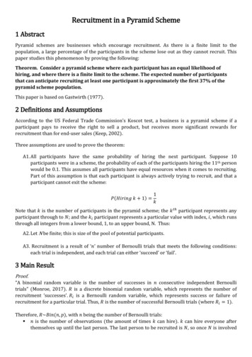
Recruitment in a Pyramid Scheme1 AbstractPyramid schemes are businesses which encourage recruitment. As there is a finite limit to thepopulation, a large percentage of the participants in the scheme lose out as they cannot recruit. Thispaper studies this phenomenon by proving the following:Theorem. Consider a pyramid scheme where each participant has an equal likelihood ofhiring, and where there is a finite limit to the scheme. The expected number of participantsthat can anticipate recruiting at least one participant is approximately the first 37% of thepyramid scheme population.This paper is based on Gastwirth (1977).2 Definitions and AssumptionsAccording to the US Federal Trade Commission’s Koscot test, a business is a pyramid scheme if aparticipant pays to receive the right to sell a product, but receives more significant rewards forrecruitment than for end-user sales (Keep, 2002).Three assumptions are used to prove the theorem:A1. All participants have the same probability of hiring the next participant. Suppose 10participants were in a scheme, the probability of each of the participants hiring the 11th personwould be 0.1. This assumes all participants have equal resources when it comes to recruiting.Part of this assumption is that each participant is always actively trying to recruit, and that aparticipant cannot exit the scheme:()Note that is the number of participants in the pyramid scheme; theparticipant represents anyparticipant through to ; and the participant represents a particular value with index, which runsthrough all integers from a lower bound, 1, to an upper bound, N. Thus:A2. Let N be finite; this is size of the pool of potential participants.A3. Recruitment is a result of ‘ ’ number of Bernoulli trials that meets the following conditions:each trial is independent and each trial can either ‘succeed’ or ‘fail’.3 Main ResultProof.“A binomial random variable is the number of successes in consecutive independent Bernoullitrials” (Monroe, 2017). is a discrete binomial random variable, which represents the number ofrecruitment ‘successes’.is a Bernoulli random variable, which represents success or failure ofrecruitment for a particular trial. Thus, is the number of successful Bernoulli trials (where).Therefore,(), with being the number of Bernoulli trials: is the number of observations (the amount of times can hire). can hire everyone afterthemselves up until the last person. The last person to be recruited is , so once is involved

in the scheme, there is no one left to recruit. Therefore, there is no probability of recruitment atN ( ends at). Therefore().is the probability of hiring such that.is a Bernoulli random variable, that can take two values: 1, when successful (hiring) and 0when failure (not hiring). Therefore, is the sum of successes for the Bernoulli trials: ()()The expectation of a binomial variable is the sum of probabilities: ( ).( ) is the expected number of people a participant can anticipate to recruit. Therefore, ( ) for theBernoulli trials between andis the sum of successes:( ) Therefore, ( ) is the sum of all probabilities of success (where), betweenentry (so the first opportunity to hire), andthe last opportunity to hire:( )the position of(1)The simplest way to demonstrate the relationship between the number of participants in the scheme,), is to draw a diagram., and the probability of hiring, (The domain is restricted tothe lower bound is the scheme’s founder;is the last agentwho can expect to recruit another agent. In other words, once is involved in the scheme, there is noone left to recruit, so there is no probability of recruitment.Fig.1Adding all the individual probabilities of success can be approximated to adding all of the ‘strips’beneath the curve in Figure 1. Therefore, integrating the curve would give an estimate for theexpected number of recruits. Note that from now on, ( ) is being approximated, this is explainedlater on and in the discussion. Therefore, ( ) can be approximated as:( )(2) Theparticipant can only recruit people who join after themselves. This is the area beneath thecurve, constrained by and the final hiring opportunity, when.Integrating (2), and inputting these bounds gives us the following:( )ln( ))( ) ln(ln( )

We re-write this expression for the expected number of people that participantrecruit as:( )ln (can anticipate to)(3)However, there are two adjustments that need to be made to this formula:Fig.2Firstly, the model excludes the probability ofrecruiting.Figure 2 shows that when, the current model would ignoreththe probability of hiring the 6 participant. This is because theprobability should have a width of 1, as is a discrete variable, on acontinuous axis. This ensures that.The solution to this is to adjust the boundaries to include , so thatthe probability of hiring the 6th participant is included:( )ln ( )(4)Fig.4Fig.3Secondly, Figure 3 shows that themodel underestimates the probabilityof hiring as the curve ‘truncates’ theprobability. Again,. So, if the height is notconsistent, and gets truncated, theprobability is underestimated.This chronic underestimation converges to the Euler-Mascheroni constant, , which roughly equals.2 as approaches . This is the sum of all the underestimations. This constant is the differencebetween the harmonic series and the natural logarithm function. [ln ]. Given a populationof 500, the truefor the first participant (between 1 and) is different from the model(ln ( )) by approximately :lnln.To reduce this error, the probability columns should be re-centred, with as their midpoints. This isshown in Figure 4. There is still an underestimation occurring, but it is less than . Equation (5) showsthis adjustment in the model:( )ln (.)(5)To check these results, we can use an example. If, what is the possibility of the 10th personthrecruiting? The 10 participant would only have one opportunity to hire and should have a 0.1probability of hiring. Thus, the expected number of recruits should be 0.1 for this participant:.( ) ln () ln ().This model is close to the true result; the small values of and have caused a moderate degree ofinaccuracy, but this example used small values for simplicity.This paper is aiming to find the number of participants that are expected to recruit at least one people.If we assume and are large, we can use Equation (4), above. The validity of this is discussed later.

To find the value ofwhen 1( ), 1( ), is substituted into the equation:ln ( )The next step is to raise to the power of both sides:Which can be rearranged to:.Therefore, the value of , for which it can be expected to recruit one or more new participants is thefirst 37% of the population.This ends the proof.This methodology can be extended for those expecting to recruit 2 or more, 3 or more, and beyond:( ).( ).4 Applying the modelFurther results can be derived using Equation (5). To do this, another assumption is added:A4. The only source of revenue is from recruiting. This follows the definition of a pyramid scheme,as many of these schemes contain worthless or overvalued products that are difficult to sell:We use Excel to generate random values for and , where, in order to estimate the expectednumber of recruits, ( ), and their expected profit, ( ). For example, inputting randomly choseninto Equation (5), the randomly chosen participant is expected torecruit 1.53 people:.( ) ln ().To join the Bull Investment Group, which was found to be an illegal pyramid scheme, the initialinvestment cost was 2,500 and the recruitment bonus was 900 (Gastwirth, 1977). Using thesefigures, and assuming A3, this participant’s expected profit can be estimated:( )( ).So, for this value of , the participant is expected to make a loss. This application can be used for othervalues of and . Figures 5 and 6 display the result of picking 10,000 random values.(Fig.5Distribution of 𝐸(𝑅) for)Position of Entry11109876543210Fig.6Distribution of 𝐸(𝛱) for( )Position of Entry 8,000.00 6,000.00 4,000.00 2,000.00 -2,000.00 000.20.40.60.8% of N1 -4,000.000.20.40.60.81% of N

It can be seen that there is exponential decay for both ( ) and ( ). For 36.56% of the simulatedpartcipants ( ), consistent with the theorem’s result of c. 37%. Only 612 of the observations hadan ( ), using the Bull Investment Group’s initial cost and recruitment benefits. To break even, aparticipant would have to recruit 2.778 people. Note that: ( ). This shows.that 6% of the population is expected to break even. Here, the simulation backs the theorem.5 DiscussionThis theorem proves that the majority of participants are unable to recruit, let alone recruit enoughnew participants to cover the costs of joining the scheme. Many of these schemes advertise incomelevels based on recruitment goals, proven to be unrealistic.However, being in the bottom 63% of the scheme doesn’t mean you can’t recruit. It could be thateveryone hires 1 person, apart from . Likewise, being in the first 37% doesn’t guaranteerecruitment. An expected value is not a defining amount, there will be natural variation from this. Thisis obvious when ( ) is not an integer; it is impossible to recruit a fraction of a person. Someparticipants will recruit more than their ( ), and some less.Throughout this paper, ( ) has only been approximated, as the natural logarithm underestimates( ). This is because the harmonic series, , is being approximated by ln , but they are notidentical. The error between the two is the Euler-Mascheroni constant, . The model in this paper will)have a smaller error as is finite [(]. The main theorem ignored . This is due to largevalues of and ; with large values, the underestimation is minimised. A significant proportion ofcomes from early values of (As seen in Figure 3). Therefore, the underestimation after 37% of N issmall. Therefore, the natural logarithm is almost identical to the harmonic form with these largevalues. This means that the adjusted Equation (5) is not required: Equation (4) is sufficient.Although this model does illustrate the difficulty of recruiting, it may do so too simplistically. Some ofthe assumptions may not be valid. Realistically, some participants will have more resources, such asmoney and time, which is likely to increase their probability of hiring. Therefore, assumption A1 is toosimple. If some participants probability of hiring was greater than , the percentage ofthat canexpect to recruit at least one person would be lower. It was also assumed that and are large, sothat Equation (4) could be used. This is usually true such as in the UK’s ‘Give and Take’ pyramidscheme which involved at least 10,000 victims (BBC News). However, sometimes pyramid schemescan be considerably smaller, so using Equation (4) would underestimate the percentage that canexpect to recruit at least one. Also, A4 may be untrue. Most pyramid schemes do have a product to sell,and despite it being difficult to sell, it is possible to have a source of revenue from products. Thus, theprofit earned by a participant is likely to be higher than the model estimates.6 References1. BBC News (2015) Promoter of 21m pyramid scam ordered to pay back 1. Available 536824 (Accessed 23/03/18)2. Gastwirth, J.L. (1977) A Probability Model of a Pyramid Scheme, American Statistician, Vol. 31, No.2, p7982.3. Keep, W.W. and Vander Nat, P. J. (2002) Marketing Fraud; An approach for differentiating multilevelmarketing from pyramid schemes. Journal of Public Policy and Marketing, pp. 139 – 151.4. Lagarias, J.C. (2013) Euler’s Consant Euler’s Work and Modern Developments, American MathematicalSociety, Vol. 50, No. 4, pp. 527-6285. Monroe, W. (2017) Bernoulli and Binomial Random Variables, Stanford University. Available df (Accessed: 08/03/2018)

Theorem. Consider a pyramid scheme where each participant has an equal likelihood of hiring, and where there is a finite limit to the scheme. The expected number of participants that can anticipate recruiting at least one participant is approximately the first 37% of the pyramid scheme population. This paper is based on Gastwirth (1977).