WIXLIB

00 101 10, the first symbol is decodedas “a” (the only codewordbeginning with 0).We remove codeword 0, and the remainingcode is 0101 10. The second symbol is similarly decoded as“a,” leaving 101 IO. For string 101 10, the only codewordbeginning with 10 is “b,”so we are left with 1 I O for c.We have described Table 1 in terms of Huffman coding.We now present an arithmetic coding view, with the aid ofFigure 1. We relate arithmetic coding to the process of subdividing the unit interval, and we make twopoints:Point I Each codeword (code point) is the sum of the probabilities of the preceding symbols.Point 2 The width or size of the subinterval to the right ofeach code pointcorresponds to theprobability of thesymbol.We havepurposelyarrangedTable 1 with the symbolsordered according to their probability p , and the codewordsare assigned in numerical order. We now view the codewordsas binary fractional values (.OW, .loo, .110 and .11 I). Weassume that the reader is familiar with binary fractions, i.e.,that ,i, and are respectively represented as .I , .O I , and . 1 1 1in the binary number system. Notice from the constructionof Table 1, and refemng to thepreviously stated Point I , thateach codeword is the sumof the probabilities ofthe precedingsymbols. Inother words, eachcodeword is a cumulativeprobability P.Now we view the codewords as points (or code points) onthe number line from 0 to 1, or the unit interval, as shown inFig. 1. The four code points divide the unit interval into foursubintervals. We identify each subinterval withthe symbolcorresponding to its leftmost point. For example, the intervalfor symbol “a” goes from 0 to . I , and for symbol “d” goesfrom . I 1 1 to 1.O. Note also from the construction of Table 1,and refemng to theprevious Point 2, that the width or size ofthe subinterval to the right of each code point corresponds tothe probability of the symbol. The codeword for symbol “a”has the interval, the codeword for“b”(. 100) has the interval,and “c” (. 1 IO) and “d”(. 1 11) each have Q of the interval.In the example data, the first symbol is “a,” and the corresponding interval on the unit interval is [O,.l). The notation“[0,.1)” means that 0 is includedin the interval, and thatfractions equal to orgreater than 0 but less than . 1 are in theinterval. The interval for symbol “b” is [.l,.l IO). Note that .1belongs to the interval for “b” and not for “a” Thus, codestrings generated by Table I which correspond to continuations of data strings beginning with “a,” when viewed as afraction, never equalor exceed the value 0.1. Data string“ a d d d d d . . . ” is encodedas “0111111 .,”which whenviewed as afraction approaches butnever reaches valueIBM J . RES. DEVELOP.VOL. 28NO. 2MARCH 19840a,100,110IllIIIIbcd4Figure 1 Codewords of Table 1 as points on unit interval.a0Icb100a,010IdIll,110hICIIIIIFigure 2 Successive subdivision of unit interval for code of Table 1and data string “a a b . . .”.lOOOOO. . We can decode by magnitude comparison;if thecode string is less than 0.1, the first data symbol must havebeen “a”Figure 2 shows how the encoding process continues. Once“a” has been encodedto [O,. l), we next subdivide this intervalinto the same proportions as theoriginal unit interval. Thus,the subinterval assigned to the second “u” is [O,.Ol). For thethird symbol, we subdivide [0,.01), and the subinterval belonging to third symbol “6” is [.OO l ,.OO l l). Note that each ofthe two leading Os in the binary representation of this intervalcomes from the codewords (Table 1) of the two symbols “a”which precede the “b.” Forthefourth symbol ”c,” whichsubintervalisfollows ‘‘a a b,” the corresponding[.0010110,.0010111).In arithmetic coding we treat thecode points, which delimitthe interval partitions, as magnitudes. To define the interval,we specify 1) the leftmost point C, and 2) the interval widthA . (Alternatively one can define the interval by the leftmostpoint and rightmost point, or by defining the rightmost pointand the available width.) Width A isavailable forfurtherpartitioning.We nowpresent somemathematicsto describe what ishappening pictorially in Fig. 2. From Fig. 2 and its description,we see that there aretwo recursive operations needed to definethe current interval. For encoding, the recursion begins withthe “current” values of code point C and available width A ,and uses the value of the symbol encoded to determine“new”values of code point C and width A . At the endof the currentrecursion, and before the next recursion, the “new” values ofcode point and width become the “current” values.New code pointThe new leftmost point of the new interval is the sum of thecurrent code point C, and the product of the interval width137GLEN G. LANGDON, JR.

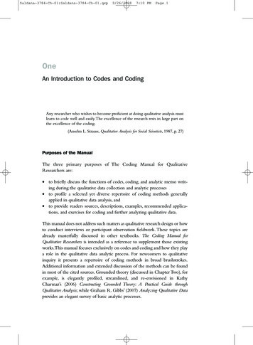
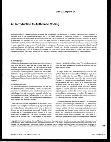
0II,,001Id-10011IaId1-Id1IIll4hIaI(IIhI c IIaI b ICIretain the important techniqueof the double recursion. Consider thearrangement of Table 2. The “codeword”corresponds to the cumulativeprobability P of the preceding symbols in the ordering.I.lFigure 3 Subdivision of unit interval for arithmetic code of Table 2and data string“a a b. . .”Table 2 Arithmeticcodeexample.SymbolCumulativeprobability PSymbolprobability pLength.oo132dba.oo1.ooo.o I 1.010.IO01C.111.oo13W of the current interval and the cumulative probability P,for the symbol i being encoded:New C Current C ( A X Pi).For example, after encoding “a a,” the current code point Cis 0 and theinterval width A is .O 1. For “ a a b,” the new codepoint is .OO I , determined as0 (current code point C), plus theproduct (.Ol) X (.loo). The factor on theleft is the width A ofthe current interval, and the factor on the right is the cumulativeprobability P for symbol “b”; see the“Cumulativeprobability” column of Table 1.New interval width AThe width A of the current interval is the product of theprobabilities of the data symbols encoded so far. Thus, thenew interval width isNew A Current AXPi,where thecurrent symbol is i. For example,afterencoding “a a b,” the interval width is ( . I ) X ( . I ) X (.Ol), which is.om I .In summary,we can systematically calculate the next interval from the leftmost point C and width A of the currentinterval, given the probability p and cumulativeprobability Pvalues inTable I for the symbol to be encoded. The twooperations (new codepoint andnew width) thus forma doublerecursion. This double recursion is central to arithmetic coding, and this particular version is characteristic of the class ofFIFO arithmetic codes which use the symbolprobabilitiesdirectly.138TheHuffman codeof Table I correspondsto a specialinteger-length arithmetic code. With arithmetic codes we canrearrange the symbols and forsake the notion of a k-bit codeword for a symbol corresponding to a probability of 2-k. WeGLEN G. LANGDON, JR.The subdivision of the unit interval for Table2, and for thedata string “ a a b,” is shown in Figure 3. In this example, weretain Points 1 and 2 of the previous example, but no longerhave the prefix property of Huffman codes. Compare Figs. 2and 3 to see that the interval widths are the same but thelocations of the intervals have been changed in Fig. 3 toconform with the new ordering in Table 2.Let usagaincodethe string “a a b c.” This examplereinforces thedouble recursionoperations, where the newvalues become the current values for the next recursion. It ishelpful to understand the arithmeticprovided here, using the“picture” of Fig. 3 for motivation.The first “a” symbol yields the code point .O 1 1 and interval[.O 1 1,.1 1 l), as follows:First symbol ( a )C N e w c o d e p o i n t C O I X(.011) .011.(Current code point plus currentwidth A times P.)A : New interval width A 1 X (.1) . l .(Current width A times probability p . )In the arithmeticcoding literature, we have called the value AX P added to the oldcode point C, the augend.The second “a” identifies subinterval [.1001,.1101).Second symbol ( a )C: New code point .011 .1 X (.011) .O 1 1 (current code point).0011 (current width A times P,or augend).lo0 1. (new code point)A: New interval width A . 1 X (.I) .O 1.(Current width A times probability p.)Now the remaininginterval is one-fourththe width of the unitinterval.For the third symbol, “6,” we repeat the recursion.Third symbol ( 6 )C: New code point .lo01 .01 X (.001) .10011.lo01 (currentcodepoint C ).OOOO 1 (current width A times P, or augend)-,1001I (new code point)A : New interval width A .01 X (.01) .0001.(Current width A times probability p.)Thus, following the codingof“ a a b,” the interval is[.loo1 1,.10101).IBM J. RES. DEVELOP.VOL. 28NO. 2MARCH 1984

To handle the fourthletter, “c,” we continue as follows.Fourth symbol (c)C: New code point .IO011 .0001X(.Ill).1010011.IO01 1(current codepoint),0000I 1 1 (current width A times P, or augend). I O 1001 1 (new code point)A : New interval width A .0001 X (.001) .0000001.(Current width A times probability p.)Carry-overproblemThe encoding of the fourth symbol exemplifies a small problem, called the carry-over problem. After encoding symbols“a,” “a,”and “b,” each having codewords of lengths1, 1, and2, respectively, in Table I , the first four bits of an encodedstring using Huffman coding would not change. However, inthis arithmeticcode, the encoding of symbol “c” changed thevalue of the third code-string bit. (The first three bits changedfrom . I O 0 to .I01 .) The change was prompted by a carry-over,because we are basically adding quantities to thecode string.We discuss carry-over control later on in thepaper.Code-string terminationFollowing encoding of “a ab c,” thecurrent interval is[.1010011,.1010100). Ifwe were to terminate the code stringat this point (no more data symbols to handle), any valueequal to or greater than ,101001 1, but less than .1010100,would serve to identify the interval.Let us overview the example. In our creation of code string.1010011, we in effect added properly scaled cumulative probabilities P, called augends, to the code string. For the widthrecursion on A , the interval widths are, fortuitously, negativeintegral powers of two, which can be represented as floatingpoint numbers with one bit of precision. Multiplication by anegative integral power of two may be performed by a shiftright. The code string for“a a bc” is the result of the followingsum of augends, which displays the scaling by a right shift:. I O 1001 I lies in [.O 1 1,. I IO), which is a’s subinterval. We cansummarize this step asfollows.Step I : Decoder C comparison Examine the code string anddetermine the interval in which it lies. Decode the symbolcorresponding to thatinterval.Since the second subinterval code pointwas obtained at theencoder by addingsomethingto .011, we can prepare todecode the second symbol by subtracting .011 from the codestring: .IO1001 1 - .011 .0100011. We then have Step 2.Step 2: Decoder C readjust Subtract from the codestring theaugend value of the code point for thedecoded symbol.Also, since the values for the second subinterval were adjusted by multiplying by .I in the encoder A recursion, wecan “undo” that multiplication by multiplying the remainingvalue of the codestring by 2. Our code string isnow .IO000 1 I .In summary, we have Step 3.Step 3: DecoderC scaling Rescale thecode C for directcomparison with P by undoingthe multiplication for thevalue A .Now we can decode the second symbol from the adjustedcodestring .IO001 1 by dealing directly with the values inTable 2 and repeating Decoder Steps 1, 2, and 3.Decoder Step 1 Table 2 identifies “a” as the second datasymbol, because the adjusted code string is greater than .01 I(codeword for “a”)but less than . I 1 I (codeword for “c”).Decoder Step 2 Repeating the operation of subtracting .O I I ,we obtain.100011 - .01I .001011.Decoder Step 3 Symbol “a” causesmultiplication by .I atthe encoder, so the rescaled code string is obtained by doublingthe result of Decoder Step 2:.01011.o 1 IThe third symbol is decoded as follows.01 100 1111.101001 IDecoder Step 1 Referring to Table 2 to decode the thirdsymbol, we see that .O I O 1 1 is equal to or greater than ,001(codeword for “b”)but less than ,011 (codeword for “a”),andsymbol “b” is decoded.DecodingLet us retain code string .lOlOOl 1 and decode it. Basically,Decoder Step 2 Subtracting out .00 1 we have .OO 1 1 1:the code string tells the decoder what the encoder did. In asense, the decoder recursively “undoes” the encoder’s recursion. If, for the first data symbol, the encoder had encoded a“b,” then (referring to the cumulative probability P columnof Table 2), the code-string value would be at least ,001 butless than .011. For encoding an “a,” the code-string valuewould be at least .O 1 1 but less than . 1 1 1. Therefore, the firstsymbol of the data string must be “a” because code-string.01011 - ,001 ,0011 I .IBM J . RESDEVELOP.VOL. 28-NO. 2MARCH 1984Decoder Step 3 Symbol “b”caused the encoder to multiplyby .O 1, which is undone by rescaling with a 2-bit shift:,00111 becomes . I 1 I .To decode the fourth and last symbol, Decoder Step 1 issufficient. The fourth symbol is decoded as “c,” whose codepoint corresponds to the remainingcode string.139GLEN G . L ANGDON. JR.

Symbol-Codeword0Ubc10II(a)well as compression codes benefit from the code tree view.Again, the code alphabet is the binary alphabet {O, 11. Thecode-string tree represents the set of all finite binarycodestrings, denoted {O,l)*.We illustrate a conventional Huffman codein Figure 4,which shows the code-stringtreeformappingdata strings “b a a c” to a binary code string. Figure 4(a) shows acodewordtable for data symbols “a,” “b,” and “c.” Theencoding proceeds recursively. The first symbol of string s,“b,” is mapped to code string 10, “b a” is mapped to codestring 100, and so on, asindicated in Fig. 4(b). Thus the depthof the code tree increases with each recursion. In Fig. 4(c) wehighlight the branches traveled to demonstrate that thecodingprocess successively identifies the underlinednodes inthecode-string tree. The root of the codeword tree is attached tothe leaf at the current depth of the tree, as per the previousdata symbol.IC)Figure 4 The code-string tree of a prefix code. Example code, imageof data string is a single leaf: (a) code table, (b) data-string-to-codestring transformation,(c) code-string tree.140At initialization, the available code space ( A ) is a set {O,l )*,which corresponds to the unitinterval. Following the encodingof the first data symbol b, we identify node 10 by the pathfrom the root. The depth is 2. The current code space is nowall continuations of code string 10. We recursively subdivide,or subset, the current code space. A property of prefix codesis that a single node in the codespace is identified as theresultof the subdivision operation. Intheunit intervalanalogy,prefix codes identify single points on the interval. For arithmetic codes, we can view the code as mapping a data stringto an interval of the unit interval, ,as shown in Fig. 3, or wecan view the result of the mapping asa set of finite strings, asshown in Fig. 4.2. A Binary Arithmetic Code (BAC)We have presented a view of prefix codes as the successiveapplication of a subdivision operation on the code space inorder to show that arithmetic coding successively subdividesthe unit interval. We conceptually associate the unit intervalwith the code-string tree by a correspondence between the setof leaves of the code-string tree at tree depth D on one hand,and the rational fractions of denominator 2D on the otherhand.A general view of the coding processWe have related a special prefix code (the symbols wereordered with respect to their probability) and a special arithmetic code (the probabilities were all negative integral powersoftwo) by picturing theunit interval. The multiplicationinherent in the encoder width recursion for A , in the generalcase, yields a new A which has a greater number of significantdigits than the factors. In our simple example, however, thismultiplication did notcause the required precision to increasewith the length of the code string because the probabilities pwere integral negative powers of two. Arithmetic coding iscapable ofusing arbitrary probabilities by keeping the productto a fixed number of bits of precision.We teach the binary arithmetic coding (BAC) algorithm bymeans of an example. We have already laid the groundwork,since we follow theencoderanddecoder operationsandgeneral strategy of the previous example. See [ 2 ] for a moreformal description.A key advance of arithmetic coding was to contain therequired precision so that the significant digits of the multiplications do not grow witb the code string. We can describethe use of a fixed number of significant bits in the setting of acode-string tree. Moreover, constrained channel codes [ 11 asThe BAC algorithm may be used for encoding any set ofevents,whatever the original form, by breaking the eventsdown for encoding into a succession of binary events. TheBAC accepts this succession of events and delivers successivebits of the code string.GLEN G L ANGDON. JRIBM J. RES. DEVELOP.VOL. 28NO. 2MARCH 1984

The encoder operates onvariable MIN, whose values are T(true) and F (false). The name MIN denotes “more probablein.” If MIN is true (T), the event to be encoded is the moreprobable, and if MIN is false (F), the event to be encoded isthe less probable. The decoder result is binary variable MOUT,of values T and F, where MOUT means “moreprobable out.”Similarly, at the decoder side, output value MOCJT is true (T)only when the decoded event is the more probable.In practice, data to be encoded are not conveniently provided to us as the “more” or “less” probable values. Binarydata usually represent bits from the real world. Here, we leaveto a statistics unit the determinationof event values T or F.Consider, for example, a black and white image of twowhitevalued pels (pictureelements) which hasaprimarybackground. For these data we associate the instances of awhite pel value to the “moreprobable” value (T) and a blackpel value into the“less probable” value (F). The statistics unitwould thus have an internal variable, MVAL, indicating thatwhite maps toT. On the other hand,if we had an image witha black background, the mapping of values black and whitewould be respectively to values T and F (MVAL is black). Ina more complex model, if the same black and white imagehad areas of white background interspersed with neighborhoods of black, the mappingof pel values black/white to eventvalues F and T could change dynamically in accordance withthe context (neighborhood) of the pel location. In a blackcontext, the black pel would be value T, whereas in the contextof a white neighborhood the black pel would be value F.The statistics unit must determine the additional information as to by how much value T is more popular than valueF. The BAC coder requires us to estimate therelative ratio ofF to the nearest power of 2; does F appear 1 in 2, or I in 4,or 1 in 8, etc., or 1 in 4096? We therefore have 12 distinctcoding parameters SK, called skew, of respective index 1through 12, to indicate the relative frequency of value F. In acrude sense, we select one of 12 “codes” for each event to beencoded or decoded. By approximating to 12 skew values,instead of using a continuum of values, the maximum loss incoding efficiency is less than 4 percent of the original file sizeat probabilities falling between skew numbers 1 and 2. Theloss at higher skew numbers is even less; see [2].In what follows, our concern is how to code binary eventsafter the relative frequencies have been estimated.The basic encoding processThe double recursion introduced in conjunction with Table 2appears in the BAC algorithm as a recursion on variables C(for code point) and A (for available space). The BAC algorithm is initialized with the code space as the unit interval[O,l) from value 0.0 to value 1.0, with C 0.0 and A 1.0.IBM J. RES. DEVELOP.VOL. 28NO. 2MARCH 1984The BAC coder successively splits the width or size of theavailable code space A , or current interval, into two subintervals. The left subinterval is associated with F and the rightsubinterval with T. Variables C and A jointly describe thecurrent interval as, respectively, the leftmost point and thewidth. As with the initial code space, the current interval isclosed on the left and open on theright: [C,C A ) .In the BAC, not all intervalwidths are integral negativepowers of two. For example, where p of event F is 4, the otherprobability for T must be i.For the width associated with Tof j , we have more than one bit of precision. The product ofprobabilities greater than f can lead to a growing precisionproblem. We solve the problem by representing space A witha floating point number to a fixed precision. We introducevariable E fo

frequent symbols with short code-string length increases, and encoding the less-frequent events with long code length in- creases. Let e, denote the occurrences of the ith symbol in a data string. For the memoryless model and a given code, let 4 denote the length (in bits) of the code-string increase associated