WIXLIB

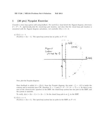
EE C128 / ME134 Problem Set 6 Solution1Fall 2011(20 pts) Nyquist ExerciseConsider a close loop system with unity feedback. For each G(s), hand sketch the Nyquist diagram, determineZ P N , algebraically find the closed-loop pole location, and show that the closed loop pole location isconsistent with the Nyquist diagram calculation. Let controller D(s) k 2.a) G(s) s 1D(s)G(s) 2(s 1). The open-loop system has no poles, so P 0.Now, plot the Nyquist diagram:Once feedback is added (k D(s)), from the Nyquist diagram, the point k1 0.5 is inside thecontour and is encircled once CW, therefore N 1 and Z P N 0 ( 1) 1. So there is onezero of the characteristic equation in the RHP, the closed-loop system has one pole in the RHP, andthe system is unstable.To verify, (s) 2(s 1) 1 2s 1. So the closed loop pole is at 12 , in the RHP.b) G(s) s 1D(s)G(s) 2(s 1). The open-loop system has no poles in the RHP, so P 0.

Once feedback is added (k D(s)), the point k1 0.5 is not inside the contour, therefore N 0 Z P . So there are no zeros of the characteristic equation in the RHP, and no poles of the system inthe RHP.To verify, (s) 2(s 1) 1 s 3. One pole at -3. No poles or zeros in the RHP, thus N 0.This corresponds to the Nyquist diagram where 1 lies outside the contour.c) G(s) 1s 1P Open loop poles in the RHP 0N CCW encirclements of k1 0Z Closed loop poles in the RHP P N 0Algebraic solution of CL poles: (s) D(s) kN (s) s 1 k.Solving (s) 0 with k 2 yields s 3. Thus, no CL poles in the RHP, and the Nyquist diagramis consistent.d) G(s) 1s 1

P Open loop poles in the RHP 1N CCW encirclements of k1 1Z Closed loop poles in the RHP P N 0Algebraic solution of CL poles: (s) D(s) kN (s) s 1 k.Solving (s) 0 with k 2 yields s 1. No CL poles in the RHP, so the Nyquist diagram isconsistent.2(20 pts) Nyquist PlotFor controller D(s) k andG(s) s 2(s 1)(s 2)(s 3)a) Hand sketch the asymptotes of the Bode plot magnitude and phase for the open-loop transfer functions.b) Hand sketch Nyquist diagram.At s 0, G(s) 13 .From there, we can see that the Nyquist diagram should go through the point -0.333. We also knowthe output contour should travel the same direction since there are poles on the left side and a zero onthe right side. The positive real intercept will occur when G(jω) 0, which can be estimated fromthe Bode plot as ω 2, which is good enough for sketching purposes.

To more accurately find the positive real intercept, one would in practice read off the value from theMatlab Bode plot. The positive intercept can also be found from:2πn 0 (jω 2) (jω 1) (jω 2) (jω 3)(1) π atan( ω/2) atan(ω/1) atan(ω/2) atan(ω/3)(2) π 2atan(ω/2) atan(ω) atan(ω/3)(3) ω 1.8708(4) G(s) 0.1333(5)(Using):x fsolve(@(x) pi-2*atan(x/2) - atan(x) - atan(x/3),[0]);s j*x;(s - 2)/((s 1)*(s 2)*(s 3))c) From Nyquist diagram, determine range of k for stability.We need to place k such that k1 is not encircled CW by the Nyquist diagram. A CW encirclementwould imply N 1 and Z 1 for the characteristic equation, and thus a closed-loop pole added tothe RHP of the system. Examining the real axis of the system, the range of k1 is from (a) to 0.333 in addition to from (b) 0.1333 to , as these ranges lie outside of the CW encirclement.Therefore, the range of stable k is (a) 0 to 3 as well as (b) 7.5 to 0. The union of these two sets is 7.5 k 3.d) Verify sketches with MATLAB and hand in.

3(20 pts) Nyquist PlotFor controller D(s) k andG(s) s 1 10)s2 (sa) Hand sketch the asymptotes of the Bode plot magnitude and phase for the open-loop transfer functions.b) Hand sketch Nyquist diagram.The interesting behavior happens when the Nyquist contour approaches the double pole at the origin.We can choose to go around the left (dotted) or right (solid) side of the poles to avoid them. If wetake the left path, the outside of the diagram (at infinite magnitude) travels CCW, whereas if we takethe right, the diagram travels CW.Case 1: Left Side of polese at originCase 2: Right Side of poles at origin

c) From Nyquist diagram, determine range of k for stability.Case 1: If we took the left (dotted) path, then there are zero crossings at and (infinitesimallyclose to) 0. P 2 since there we placed the two poles in the Nyquist contour. Between 0 and there are two CCW encirclements where N 2 and thus Z 0 and the system is stable.On the positive real axis, there is only one CCW encirclement and thus the closed-loop systemhas an unstable pole for k 0. Therefore, the stable range of k is between 0 and .Case 2: If we took the right (solid) path, then there is one zero crossing infinitesimally close to 0.P 0 since there are no open loop poles in the Nyquist contour. If k1 0, then there areno encirclements and N Z 0, and the system is stable. If k1 0 then there is one CWencirclement, N 1, Z 1, and the system is unstable. These are the same ranges as the firstcase, and the range of stable k is between 0 and .d) Verify sketches with MATLAB and hand in.The Nyquist plot from MATLAB is misleading since it doesn’t include the behavior close to the zeropoles.4(20 pts) Nyquist PlotFor kD(s) 1 andG(s) (s 2)2(s 1)3 (s 4)2

a) Hand sketch the asymptotes of the Bode plot magnitude and phase for the open-loop transfer functions.Normalize the components of the transfer function:(s 2)2 (s 1)3 (s 4)2 2s 12 !2 1s 1 314 s41 1!2 14 s 12 !2 1s 1 3s41 1!2From this we can see:DC gain is 14 12 dB.There are two zeros with breakpoint at 2.There are three poles with breakpoint at 1 and two poles with breakpoint at 4.All of those breakpoints are within one decade of each other, so this diagram is going to be crowded.

b) Hand sketch Nyquist diagram.For this diagram, we will use the Bode plot information for the section of the test contour that is on the jω axis. Note that for this diagram we are using the technique where points that are infinitesimallyclose to the origin (b, c, d) are drawn a small distance away so that the phase is visible.c) From Nyquist diagram, determine range of k for stability.There are two regions of interest on the negative real axis of the Nyquist diagram. In the drawingabove they are marked with a square and a triangle. We need to find the intersection with the realaxis that divides these two regions. There are several methods we can use. Estimate from the Bode plot. The phase plot shows that ]G(jω) 180 when ω 4.The magnitude plot shows that G(j4) 40 dB 0.01. Therefore, the intersection is atapproximately 0.01. Estimate ω from the Bode plot, then calculate G(jω) . As before, ω 4 from the phaseplot.G(j4) 0.00885 0.00171j 0.00892This answer shows that G(j4) isn’t really that close to the real axis. Our approximation of theintersection is 0.00892. Start with ω 4 and use trial and error to dial it in.G(j4) 0.00885 0.00171jstartG(j3) 0.01640 0.00120jcrossed the real axisG(j3.5) 0.01190 0.000837jcrossed the real axisG(j3.3) 0.01350 0.000214jdidn’t crossG(j3.1) 0.01536 0.000651jcrossed, but got further awayG(j3.2) 0.01440 0.000184jdidn’t crossG(j3.25) 0.01394 0.000023jcrossed, got closerG(j3.24) 0.01403 0.000017jcrossed. close enough!

Take the absolute value: G(j3.24) 0.01403: to finalize the estimate: the crossing is at 0.01403. Use MATLAB’s x-y picker to get these values off the Bode or Nyquist plot. Be careful:unless you do some fancy tricks, your picked values might not be very accurate. I got ω 3.17,and the intersection at 0.0147, when I tried it. Solve G(jω) x, with negative real x, for ω.(s 2)2(s 1)3 (s 4)2s2 4s 4 5s 11s4 43s3 73s2 56s 16 ω 2 4jω 4G(jω) 54jω 11ω 43jω 3 73ω 2 56jω 16G(s) Multiply top and bottom by the complex conjugate of the denominator. ω 2 4jω 4 jω 5 11ω 4 43jω 3 73ω 2 56jω 16jω 5 11ω 4 43jω 3 73ω 2 56jω 16 jω 5 11ω 4 43jω 3 73ω 2 56jω 16The denominator is something huge, but it’s real, so we discard it. We want the numerator to bereal.N jω 7 ω 6 3jω 5 55ω 4 64jω 3 84ω 2 160jω 64Isolate the terms with j and force them to cancel. Ignore the terms without j. 0 j ω 7 3ω 5 64ω 3 160ω 0 ω ω 6 3ω 4 64ω 2 160One solution is ω 0, but we already knew about that one (it’s on the positive real axis).There’s another solution that we have to find! Since this polynomial is even it’s really a cubic.Unfortunately, cubics are pretty hard. We can use MATLAB’s roots command to find:ω 3.2442357G(jω) 0.013996In summary: depending on the method you use, your value for the intersection on the negative realaxis should be something like 0.014.Now we need to interpret the Nyquist diagram in these two regions (marked with a square and atriangle on the diagram above).Triangle region: k1 0.014:P Open loop poles in the RHP 0N CCW encirclements of k1 0Z Closed loop poles in the RHP P N 0Stable.Square region: 0 k1 0.014:P Open loop poles in the RHP 0N CCW encirclements of k1 2Z Closed loop poles in the RHP P N 2Unstable.Solving for k, we find thatk (0, 71.45) stablek (71.45, ) unstableNormally we only consider positive k. If you searched for stability conditions on negative k, you wouldfind that N 1 on the real axis before s 0.25, and N 0 afterwards. Therefore:k ( , 4) unstablek ( 4, 0) stableHowever, this is not a required part of the solution.

d) Verify sketches with MATLAB and hand in.Bode DiagramNyquist Diagram0.20.15 500.1 100Imaginary AxisMagnitude (dB)0 15000.050Phase (deg) 0.05 90 0.1 180 0.15 270 110011021010 0.2 0.2 0.15 0.1 0.05Frequency (rad/s)500.050.1Real Axis(20 pts) Gain and phase marginA closed loop system with unity gain has loop transfer functionG(s) 125(s 1)(s 5)(s2 4s 25)a) Plot the Bode magnitude and phase plots for the open loop system (MATLAB ok).Bode DiagramGm Inf dB (at Inf rad/s) , Pm 42.1 deg (at 11.4 rad/s)Magnitude (dB)500 50Phase (deg) 100900 90 180 210 110011010Frequency (rad/s)2103100.150.20.250.3

b) Determine the gain and phase margin.MATLAB’s margin command provides these values, or they can be determined graphically from theBode plot.Gain margin: Phase margin: 42.1 c) Assuming a second order approximation for the closed loop system, estimate the transient response fora step input from the phase margin and gain margin. (That is estimate ξ, overshoot, peak time, andsettling time.)Our approach is to find an open-loop second-order system whose phase and gain margins match thosefound in part (b), and then estimate the transient response parameters for the closed-loop system fromthis approximation. The OL second-order system is characterized by ξol and ωn ol, so our first step isto estimate those two parameters.We will examine two approximation methods for the second order system. Example 10.13, - 6dBBy definition, the closed loop bandwidth ωn is the frequency where the magnitude of the responseof the closed loop system is -3 dB. Following example 10.13 in Nise, for unity gain feedback, (withphase in range -135 to -225 degrees), the open loop system would have magnitude response -6 dBat this ωn . From the Matlab plot, the -6dB frequency ωn 16.The CL ξ may be estimated using the “small ξ” approximation discussed in class:(deg)ξ ΦM 0.421100or via the relationship in section 10.10 of Nise:2ξΦM tan 1 qp 2ξ 2 1 4ξ 4which proceeds as follows:qp 2ξ 2 1 4ξ 4 2ξ p(0.9022)2 2ξ 2 1 4ξ 4 4ξ 2p1 4ξ 4 (4 2 · 0.90222 )ξ 2tan ΦM1 4ξ 4 31.674ξ 41ξ4 27.674ξ 0.4360Either method is fine; obviously the results are very similar.So this closed loop estimate has ωn 16 and ξ 0.44. Approximate open loop 2nd order systemFor a second order system, we know that the phase at ωn is 90 . Here phase is 90 at ωn 6.3from the Bode diagram. We know that G(jωn ) 2ξ1ol which from the Bode plot is 10 dB ( 3),thus ξol 0.17.Therefore, our second order approximation of the open loop TF is:40s2 2.14s 40Since we are interested in the closed loop step response, we apply theG(s)1 G(s)feedback formula: