WIXLIB

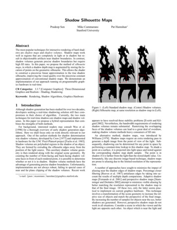
OOOAABCFigure 3: Generation of silhouette map using quadrangles. (A) linesegments with quadrangles shown in lighter color, (B) intersectiontest between line segments and rasterized fragments, (C) generatedpoints of silhouette map.Generating the Silhouette MapThis pass rasterizes the silhouette edges into the silhouette maptexture as shown in Figure 3. The rasterization rules used whendrawing wide lines vary between implementations and often do notguarantee that every pixel intersected by a line segment will be rasterized. To avoid problems due to these inconsistencies, we drawthe region around the line segment as a quadrilateral. The size ofthe quadrilateral is chosen to guarantee that a fragment is generatedfor every texel intersected by the line segment. To draw the quad,we simply offset the vertices on either side of the line by a smallamount in screen space perpendicular to the direction of the line.We also make the quads slightly longer than the line segment toguarantee that the end points of the line are rasterized as well.Since the quadrilateral is chosen conservatively, fragments thatdo not overlap the line segment may also be generated. The fragment program that selects the point on the line segment must makesure the point is actually inside the texel. To perform this test, wepass the two endpoints of the line segment as vertex parameters tothe fragment program. If one of the vertices is inside the texel,we know trivially that the line segment intersects the square andwe store the vertex into the silhouette map — see Figure 4(A). Ifneither vertex is inside the texel square, we test to see if the lineintersects the texel by intersecting the line segment with the twodiagonals of the texel. If the line intersects the texel, at least onediagonal will be intersected inside the square. If only one of thetwo intersections is inside the square we store it in the silhouettemap, and if both are valid we store the midpoint between them,as shown in Figures 4(B) and 4(C), respectively. If the diagonalsare both intersected outside the square, the line does not intersectour texel and so we issue a fragment kill, preventing the fragmentfrom being written into the silhouette map. This case is shown inFigure 4(D). This simple technique selects a point on a line segment clipped to the texel boundary, and can be implemented in anARB fragment program.To ensure enough precision, we represent the coordinates of thesilhouette points in the local coordinate frame of the texel, with theorigin at the bottom-left corner of the texel. In the fragment program, we translate the line’s vertices into this reference frame before performing our intersection calculations. In addition, we alsowant to ensure that only visible silhouettes edges are rasterized intothe silhouette map. To do this properly, the depth of the fragment iscompared to that of the four corner samples. If the fragment is farther from the light than all four corner samples, we prevent it fromwriting into the silhouette map by issuing a fragment kill.CDFigure 4: Intersection of line segment with texel. We label the pointthat will be stored in the silhouette map as “O.” (A) If either vertexis inside the texel, store it. (B) Segment intersects diagonals at onlyone point. (C) Segment intersects diagonals in two places so storethe midpoint. (D) No intersection at all, so do not store anything.The first pass, rendering a depth map of the scene from the pointof view of the light, proceeds much as in conventional shadowmaps. However, we use a simple fragment program at this stageto copy the depth output into a color output so we can read it backin subsequent passes. This is needed because our hardware doesnot allow fragment programs to bind a depth texture directly.3.1BOA1234BCFigure 5: (A) We want to shade point “O” using silhouette mappoints shown in gray. (B) We must first determine which “skewed”quadrant (1–4) the point is in. (C) We test against the eight pieshaped regions. Here we determine the point is in quadrant 1, sowe shade it based on the depth sample at the top-left corner.Finally, our implementation must handle the case where the silhouette line passes through the corner of a texel. In these situations,problems occur if we store the point in only one of the texels adjacent to the corner. To avoid artifacts and ensure the 4-connectednessof our representation, we store lines that pass near corners (withinlimits of precision) in all four neighboring texels. To do this, theclipping square is enlarged slightly to allow intersections to be validjust outside the square region. When the final point is computed, thefragment program clamps it to the texel square to ensure that all thepoints stored in a texel are always inside the texel.The algorithm was implemented as an ARB fragment programof 60 instructions, four of which are texture fetches to get the required depth samples.3.2Shadow renderingIn this pass we decide if a point is in shadow using the depth andsilhouette maps. The depth tests are first performed and if they allagree we shade the point based on their result. If they disagree, thesilhouette map is used to approximate the shadow edges passingthrough this texel and shade the point accordingly.Line segments between the current point and these four neighbors divide the texel into four “skewed” quadrants, as shown inFigure 5. Each quadrant is shaded in the same manner as its cornerpoint, so we must determine which quadrant the current fragmentis in to properly shade it. We divide the texel into eight pie-shapedregions (two for every quadrant) and perform simple line tests toplace the point in the correct quadrant. The fragment is then shadedappropriately based on the result of the quadrant’s depth test.This step of the algorithm is implemented in 46 instructions ofan ARB fragment program. The remaining instructions are used toshade the fragment. There are a total of nine texture fetches in theshadow determination portion, four to gather the depth samples andfive to get the silhouette point and its neighbors.

Figure 6: Test scenes (standard shadow map on the left, silhouettemap on the right). From top to bottom: C ROWD , J EEP, C ASTLE .4ResultsWe test the silhouette map algorithm using the scenes shown inFigure 6. These scenes are dynamic and the silhouette map is recomputed for every frame. Statistics for these scenes are given inTable 1. The first scene, C ROWD , consists of twenty-four characterscasting shadows onto a distant wall. When viewed from certain directions, the depth complexity of the shadow volumes in this sceneis very high. The second scene, J EEP, and the third scene, C AS TLE , are examples typical of interactive entertainment applications.We also experiment with another scene, S TRIKE , to illustrate shadows on curved objects (see Figure 9). Here, each bowling pin istessellated to 450 triangles.For these figures, the shadow and silhouette maps are generatedat a resolution of 512 by 512 texels. In all test scenes, there is substantial improvement in shadow quality between standard shadowmaps and silhouette maps. Our tests also indicate that the problemswith depth bias are no worse in silhouette maps than shadow maps.We also compare silhouette maps to an implementation ofshadow volumes based on NVIDIA’s publicly available shadow volume demo [Kilgard 2000]. This code identifies silhouette edges andextrudes shadow volumes. We test the two implementations on thescenes C ROWD, J EEP and C ASTLE. The quality of shadows computed using silhouette maps is similar to that of shadow volumesand the frame rates are comparable. In both algorithms, the actualframe rate is limited by the geometry issue rate of the applicationrunning on the host.Although the silhouette map algorithm requires more arithmeticoperations than the other algorithms, it is more important to compare the bandwidth requirements of the algorithms. We develop asimple model for the bandwidth consumed by all three algorithms,and measure scene statistics in order to compare them.First, we compare shadow maps to silhouette maps. In the generation step, both algorithms generate a depth. Silhouette maps alsorequire the silhouette be drawn. However, there are many fewersilhouette texels than interior texels, so the incremental cost of silhouette maps is small.During shadow determination, shadow maps read 1 depth value.This is really the worst case, since for a magnified shadow map lessthan 1 depth value is read on average. Although silhouette maps use4 neighboring depth values, on average only one value is read because of the spatial locality of texture accesses. This is similar to thecase of mipmaps, which typically require only 1 texel to be read onaverage [Hakura and Gupta 1997]. To shade points near the silhouette edge, we need to read 5 silhouette points (the current silhouettepoint plus the 4 neighbors). There is less spatial locality in this casesince the silhouette is a curve, so we will assume on average 3 silhouette points will be read. Thus, the average bandwidth for depthvalues will be 4 bytes per pixel, and the average bandwidth for vertices will be 24P, where P is the percentage of pixels on silhouettes.If P 16 16%, then silhouette maps will consume less than twicethe bandwidth of shadow maps. The results in the table show thatthis is always the case. It should be noted that P is artificially highin the table because the statistics correspond to cases where we arezoomed in on the shadow. We conclude that silhouette maps andshadow maps consume roughly the same bandwidth.Next, we compare shadow maps to shadow volumes. As statedpreviously, shadow volumes require high fill rates; in our testscenes, the number of shadow volume fragments is between 4 and155 times the number of rendered pixels. We call this the overdraw factor O. To compute the bandwidth requirements, we assumeeach shadow volume fragment must read 1 depth value and 1 stencil value (1 byte). If the shadow fragment passes the depth test,the stencil value is incremented and stored in the stencil buffer; thisconsumes on average an additional 1/2 byte of bandwidth. Thus, theratio of stencil volume to shadow map bandwidth is O 5.54 . Therefore, if O 4/5.5, the shadow volume algorithm will consumemore bandwidth than the shadow map algorithm. In the scenes wetested, this is always the case.5DiscussionWe conclude by comparing silhouette maps to existing methods aswell as discussing the artifacts and limitations of our technique. Inaddition, we discuss the connection between the silhouette map anddiscontinuity meshing and propose future work.Comparison with existing techniques:Silhouette maps offer improved visual quality over conventional shadow maps.They are also complementary to Stamminger’s perspective shadowmaps. While Stamminger’s technique optimizes the distribution ofshadow samples to better match the sampling of the final image,our technique increases the amount of useful information providedby each sample. The two techniques could be easily combined toyield the benefits of both.While we have shown that silhouette maps use substantiallyless bandwidth than shadow volumes, our implementation did notshow improved performance. Currently, both our prototype and theshadow volumes implementation are limited by the speed at whichwe can generate the silhouette, which is done on the host. In addition, our algorithm was implemented using the first generationof fragment shaders. In contrast, shadow volumes benefit from established, carefully-tuned hardware paths supporting stencil bufferoperations. In the next section, we will discuss ways in which ouralgorithm could benefit from greater hardware support.

Scene NameC ROWDJ EEPC ASTLEScene InformationTrianglesSilhouette edges14,8364,8001,7327291,204466Scene Fill148.9k298.3k268.5kShadow Mapsfps11.57597fps9.27295Shadow VolumesVolume ette MapSilhouette fillP19.8k13.3%37.5k12.6%19.20k7.2%Table 1: Performance comparison of the three techniques. The scene information lists the number of triangles in each scene as well as thenumber of silhouette edges processed by the shadow volumes and silhouette map techniques. The fill-rate columns indicate the number offragments written in each algorithm for various steps. Scene fill is the number of fragments rendered to draw the scene without shadows.Volume fill is the number of fragments drawn when rendering the shadow volume geometry. The ratio of volume fill to scene fill is theoverdraw factor O. For shadow and silhouette maps the fill rate is the scene fill. The silhouette fill is the number of fragments that passthrough silhouette; P is the corresponding percentage of scene fill.Figure 7: Artifacts of our algorithm. The top row shows silhouettesand selected silhouette points, the bottom row shows the shadowsdetermined by our algorithm. (Left) two silhouettes intersect at apixel, (Center) two silhouettes pass through a pixel but do not touch,(Right) a sharp corner is lost because of depth sampling resolution.Hardware support: There are three parts of the algorithm thatcould be accelerated in hardware: Currently, we determine potential silhouette edges using codefrom the NVIDIA shadow volume demo [Kilgard 2000]. Inour results, the performance of both silhouette maps andshadow volumes was limited by the cost of this silhouette determination on the host. Both methods would benefit from afaster mechanism for determining potential silhouette edges. In generating the silhouette map, our current implementationmust draw thin quads and use a fragment program to identifythe silhouette points. One could imagine a rasterization modethat implemented this process directly. When determining shadows, our fragment program must perform unnecessary operations because of the lack of conditional execution at the fragment level. Conditional executionof arithmetic and texture fetches could reduce the work ofeach shading pass by nearly a factor of four.Eventually, one could imagine supporting the entire silhouette mapalgorithm as a primitive texture operation.Artifacts: By choosing to store only a single silhouette point ineach texel, we have limited the complexity of the curves that can berepresented in the silhouette map. For example, when two disjointsilhouettes pass through a single texel, it is not possible to store asingle point that is representative of both contours (see Figure 7).Because of the fixed resolution of the silhouette map, silhouetteswith high curvature at the texel level will have artifacts. Increasing the tessellation of the geometry, however, does not affect thevisual quality. In practice we found the artifacts introduced to beacceptable (see Figure 8) especially when considering the substantial improvement in quality relative to conventional shadow maps.Figure 8: A closeup reveals artifacts of our algorithm when the resolution of the silhouette map is too low. (Left) standard shadowmap and associated artifacts. (Center) Shadow volumes yields correct shadow. (Right) Silhouette map at the same resolution as theshadow map shows artifacts. In this case, the fender of the jeepyields an artifact like that in the center diagram of Figure 7.Discontinuity Mesh: We have presented a new algorithm that extends shadow maps by providing a piecewise-linear approximationto the silhouette boundary. This method is easy to describe as a 2Dform of dual contouring. Alternatively, we can think of the silhouette map algorithm as similar to discontinuity meshing of a finiteelement grid. We start with a regular grid of depth samples – theshadow map – where each grid cell contains a single value. We locally warp this grid so that the boundaries of grid cells are alignedwith discontinuities formed by the shadows (See Figure 10). Thisis what our algorithm allows us to do using fragment programs onthe graphics hardware. Note that when silhouette map points are atthe center of the texels, the regular grid is undeformed, leading tobehavior identical to that of conventional shadow maps.Alternative Silhouette Representations: Prior to adopting a single point as the silhouette map representation, we explored twoother techniques: triangle lists and edge equations. Initially, weconsidered using Haines’ light buffer [1986], which stores a list ofthe potential shadowing triangles for each texel. We used a fragment program ray tracer to test shadow rays against this list of triangles [Purcell et al. 2002]. Unfortunately, even for simple scenes,we found we needed a long, variable-length list of triangles to getgood results. This introduced many consequences which made itimpractical. We next investigated using line equations to approximate silhouettes. Unfortunately, it was difficult to maintain continuity between the line segments. In the end, we stored points alongthe silhouette edge in our map as described in our paper. We storeonly two parameters (the relative x and y offsets) per silhouette maptexel. Had the hardware allowed it, it would have been enough to

Figure 9: (Left) Scene rendered using a standard shadow map. (Middle) A visualization of the silhouette map superimposed on top of thescene. The red circles indicate the positions of silhouette points. On the edge of the bowling pin they are elongated into ellipses because theyare being projected from the point-of-view of the light. (Right) Scene rendered using the silhouette map.Mike Cammarano was supported by a 3Com Corporation StanfordGraduate Fellowship and a National Science Foundation Fellowship.ReferencesFigure 10: Silhouette maps can be thought of as warping a regulargrid so that grid lines align with boundaries in the geometry. (Left)The two grids. In the background, shown in dotted lines, is the silhouette map texture. In the foreground is the depth map offset by(1/2, 1/2). The large circles indicate the depth values. Superimposed on that is the silhouette, drawn in black. (Right) We warp ofthe depth map grid so that it better matches the silhouette.store a single byte to encode both of these offsets since 4 bits peroffset would be enough resolution to faithfully represent points onthe silhouette edge.Future Work: Silhouette maps offer several directions for futureresearch. A thorough exploration of different silhouette representations might yield insight into better representations for specificgeometries. In addition, one might consider extending ou

counting the number of front-facing and back-facing shadow vol-ume faces in front of each rendered point, it is possible to determine whether or not it is in shadow. Shadow volume methods have the advantage of generating p