Transcription
PharmaSUG 2017 - Paper HT03Survival 101 - Just Learning to SurviveLeanne Goldstein and Rebecca Ottesen, City of Hope, Duarte, CAABSTRACTAnalysis of time to event data is common in biostatistics and epidemiology but can be extended to avariety of settings such as engineering, economics and even sociology. While the statistical methodologybehind time to event analysis can be quite complex and difficult to understand, the basic survival analysisis fairly easy to conduct and interpret. This workshop is designed to provide an introduction to time toevent analyses, survival analysis and assumptions, appropriate graphics, building multivariable models,and dealing with time dependent covariates. The emphasis will be on applied survival analysis forbeginners in the health sciences setting.INTRODUCTIONIn most statistics academic settings, Survival Analysis is a one to two semester course that is dense withmethodology and notation. In this presentation we offer a simple way to approach time to event datawhich can be useful to those who have never taken a course in survival analysis or for those who need abit of a refresher. This presentation begins with examining the data and deciding between parametric(Accelerated Failure Time) and semi-parametric (Cox Proportional Hazards) models. We will covertesting interactions and time-dependent covariates as well as how to verify that the model assumptionsare met. We will also demonstrate useful graphing techniques for generating presentation or manuscriptquality survival plots. This workshop uses the German Breast Cancer Study (GBCS) Data from AppliedSurvival Analysis: Regression Modeling of Time to Event Data: Second Edition (Hosmer, Lemeshow, andMay 2008) and evaluates covariates that are predictive of time to breast cancer recurrence. This GBCSdata set can be found at the textbook site ftp://ftp.wiley.com/public/sci tech med/survival.EXAMINING SURVIVAL DATA - KAPLAN-MEIER METHODFirst, we examine the data using PROC LIFETEST. This procedure can be used to compute survivalestimates using the Kaplan-Meier method and the actuarial method. In our example, we study therectime variable, which estimates for each patient, the number of days from date of diagnosis to anevent, which in this disease free survival analysis is date of recurrence (or death), or number of days todate of last contact. If the date of last contact is used, and the patient has not had a recurrence during thetime they were observed, then the patient’s data is considered right censored. The Kaplan-Meier methodwill be used to estimate the cumulative proportion of patients surviving over time due to the censoredobservations not being organized in specific time intervals (more typical for the actuarial method).PROC LIFETEST DATA gbcs;TIME rectime*censrec(0);RUN;The first line of PROC LIFETEST includes a specification of the dataset. Next we use the TIMEstatement. In this statement, we write the time to recurrence (days) variable rectime and the censoringvariable censrec. The censrec variable is coded 1 if a patient had an event and 0 when the patient iscensored, i.e. has had no recurrence during the time observed. We put 0 in parentheses to indicate thevalue for the censored patients in the study. The output of PROC LIFETEST gives the following outputshown in Output 1.1
Survival 101 – Just Learning to Survive, continuedOutput 1. Partial output from PROC LIFETEST2
Survival 101 – Just Learning to Survive, continuedOutput 1 shows the results from PROC LIFETEST. First, the output shows a portion of the Product-LimitSurvival Estimates, or life table, produced by PROC LIFETEST. In this table, the first column lists timefrom 0 to the last observed time point: 2,659 days. The * indicates a patient who is censored andtherefore their rectime is the last day that they were observed. Observations without the * had an eventat their time point. The survival column shows the conditional probability of no recurrence given thepatient has made it to the rectime point without recurrence. The failure column is the compliment of theSurvival column or 1- Survival showing the probability of recurrence given the patient has not recurredyet. The Survival Standard Error provides an estimated standard error for the estimate in the survivalcolumn. The Number Failed column indicates the number of patients that have recurrence/death at therectime day. The Number Left column gives the number of patients that are still being observed andhad not yet had recurrence/death or were censored at the rectime time point.How do we interpret these results? For example, at rectime day 1807.0, the probability of not having arecurrence/death (Survival) equals 0.4994. This is the day when the probability of failure is closest to andjust greater than 50%, otherwise known as the median survival time. This is an important statistic for timeto event data and is also reported in the Quartile Estimates Table for Percent 50. Note that at rectime 1814, there are two patients who had an event which means that the Survival and Failure columnscontain missing data for the first occurrence where rectime 1814 but data are filled in for the secondoccurrence where rectime 1814. The last observation of this table, rectime 2659 days, iscensored.The quartile estimates table lists the estimated number of days when approximately 25%, 50%, and 75%of the patients have had a recurrence. Note that there is no 75% point estimate because at the lastobserved time point rectime 2659 days, failure 0.6572 or probability of recurrence 65.7%. Thismeans that the failure percentage never reaches 75% and this point estimate cannot be provided. Underthis table the mean is reported and a note is given that indicates the mean survival and standard error areunderestimated. The skewed right tendency of censored time data demonstrates why median survival ismore often requested that mean survival.The plot of Survival Probability against Time to Recurrence is called a Kaplan-Meier Curve. From thiscurve, we can observe that with increasing number of days of time to recurrence, the survival probabilitydecreases. The markers on the Kaplan-Meier Curve show when there were censored observations.In the Summary of the Number of Censored and Uncensored Values Tables, we observe that 56.41% ofthe cohort was censored. This equates to 100% - 56.41% 43.59% of the patients in this sample havinga breast cancer recurrence or death.UNIVARIATE SURVIVAL ANALYSESAfter getting summary information about the disease free survival or time to recurrence for the cohort, wemight wish to understand what covariates are predictive of time to breast cancer recurrence. Differenttechniques are used for evaluating categorical and continuous variables.TESTING CATEGORICAL COVARIATESFor categorical variables we can look at the Kaplan-Meier curves, stratifying on the covariate of interest.Here we will look at grade to see if it is associated with time to recurrence.PROC LIFETEST DATA gbcs NOTABLE;TIME rectime*censrec(0);STRATA grade / TEST LOGRANK ADJUST SIDAK;RUN;In the first line of PROC LIFETEST we add the NOTABLE option. This suppresses the life table andsummary table of quartiles. We add the STRATA statement with the covariate we wish to evaluate,grade. To quantifiably test the difference among the Kaplan-Meier curves, we use the log-rank test and3
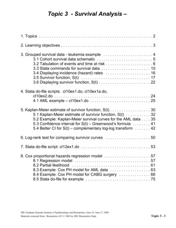
Survival 101 – Just Learning to Survive, continuedspecify TEST LOGRANK as an option in the STRATA statement. The grade covariate has three levels.Therefore, we wish to adjust the results of the log-rank test for multiple comparisons using theADJUST SIDAK option. The results of stratifying rectime by grade are show in Output 2.Output 2. PROC LIFETEST partial output for using STRATA gradeThe three Kaplan-Meier Curve plots in Output 2 allow us to evaluate the association of time to recurrencerectime with the categorical covariate grade. In the first summary table of the output, we can observethe number of failed and the number of censored at each level of the strata. The Test of Equality over4
Survival 101 – Just Learning to Survive, continuedStrata table has the results of the log-rank test. With a p-value 0.05, the log-rank test is statisticallysignificant indicating that time to recurrence rectime is significantly associated with grade. In theAdjustment for Multiple Comparisons for the log-rank test, the Sidak p-values show that there is astatistically significant difference between grade levels 1 and 3, but not between grade levels 2 and 3nor between grade levels 1 and 2. The plot of Kaplan-Meier curves demonstrates the differences inrectime among the grade levels. When there is good separation among the curves then there is asignificant difference in time to recurrence for the different levels of the covariate. When there is littleseparation or overlap among the curves then the categorical covariate is not associated with time torecurrence. In this figure, we see overlap between the red line (grade 2) and green line (grade 3) whichindicates that they are not significantly different. The Kaplan-Meier curves for grade levels 1 (blue) and 2(red) appear further apart for the most part as well as the curves for grade levels 1(blue) and 3 (green).However, the Sidak multiple comparison results indicate that levels 1 and 3 are significantly different butlevels 1 and 2 are not. This demonstrates that it is not enough to look at the plots and overall Log-Ranktest for evaluating the strata, we need to also look at the multiple comparison results.In another example, we show the results of testing the menopause (yes/no) covariate. Here we don’tneed the ADJUST SIDAK option because there are only two levels of the covariate therefore adjustingfor multiple comparisons in unnecessary. We also create a Yes/No format for menopause which makesthe plot easier to interpret.PROC FORMAT;VALUE ynf1 'No'2 'Yes';PROC LIFETEST DATA gbcs NOTABLE;TIME rectime*censrec(0);STRATA menopause / TEST LOGRANK;FORMAT menopause ynf.;RUN;The output for the stratifying rectime by menopause is in Output 3.Output 3. PROC LIFETEST partial output for using STRATA menopause5
Survival 101 – Just Learning to Survive, continuedOutput 3 shows the results of stratifying the rectime Kaplan-Meier curves by the covariate menopause.The first summary table shows the number of failed and censored in each of the two strata formenopause. The percent censor rates are similar in the two levels of menopause. The Tests of Equalityover Strata for menopause show a non-significant Log-Rank test p-value, greater than 0.05. Therefore,there is no statistically significant difference in the rectime Kaplan-Meier curves when stratified bymenopause. This non-significance is also demonstrated in the plot which shows a great amount ofoverlap in the menopause no (blue) and yes (red) Kaplan-Meier curves.Suppose now we want to evaluate the association of continuous covariates with rectime. Since theKaplan-Meier curves cannot be stratified by continuous covariates, we have two possible solutions. Firsta continuous variable could be defined into meaningful groups and then tested as above for a categoricalvariable. Second we could evaluate the continuous covariate in the Cox Proportional Hazard Model.COX PROPORTIONAL HAZARD MODELThe Cox Proportional Hazard Model is a semi-parametric model often used to for time to event data whichcan be used when the underlying distribution of the time to event data is unknown -- often the case withhealth sciences data. In a Cox Proportional Hazard Model, the hazard, or rate of failure, is modeled as afunction of the linear combination of the covariates. Similar to logistic regression which looks at theexponentiated covariate coefficient as an odds ratio, the Cox Proportional Hazard Model speaks of theexponentiated covariate coefficient as a hazards ratio. In order to use a covariate in the Cox ProportionalHazards Model, we need to make sure that two assumptions are satisfied. When the linearity assumptionis satisfied, we assume that there is a linear association between the covariate and the Cox ProportionalHazards Model outcome. And for the proportionality assumption, we assume that over time hazards ratiostay the same.TESTING CONTINUOUS COVARIATESSince we cannot use Kaplan-Meier plots and PROC LIFETEST, we instead use PROC PHREG andevaluate the significance of a continuous covariate in the Cox Proportional Hazards Model. In this section,we also evaluate that the linearity assumption and proportional hazards assumption are held.The following code evaluates the univariate association of tumor size (mm), the variable named size,with time to recurrence rectime.PROC PHREG DATA gbcs;MODEL rectime*censrec(0) size;ASSESS VAR (size) PH / RESAMPLE SEED 12345;RUN;Note that the statements for PROC PHREG are very similar to those used PROC LIFETEST. In PROCPHREG, instead of a TIME statement, a MODEL statement is used. And instead of specifying thecovariate in a STRATA statement, the covariate, size, is written in the MODEL statement after the equalsign. There is an additional ASSESS statement used in this procedure. This ASSESS statement checksfor any major issues with the linearity assumption (called functional form) and also for the proportionalhazard assumption -- that the covariate is linearly associated with the hazard for rectime and that thehazard ratio does not change with rectime. To check the linearity assumption we specify the covariatename VAR (size) in the ASSESS statement. To check the proportional hazards assumption, wespecify PH in the ASSESS statement. This ASSESS statement generates two plots: a plot of thecumulative Martingale residuals against the covariate to test the linear assumption and the plot of thestandardized score process (a Martingale residual transform) against time to recurrence rectime tocheck the proportional hazards assumption. Details about Martingale residuals or standardizes scoreprocesses are not covered in this paper. We are mainly interested in the interpretation of these plots. Forfurther information please refer to (Lin, Wei, & Ying, 1993). The RESAMPLE option in the ASSESSstatement generates a p-value for the maximum residual in each of the plots. Since this plot is based on6
Survival 101 – Just Learning to Survive, continuedsimulations using a random number generator, we set the SEED to 12345 in order to be able toreproduce the similar plots at a later time point. The partial results of the PROC PHREG for thecontinuous covariate size are provided in Output 4.Output 4. Partial Output from PROC PHREG Univariate Test for SizeIn Output 4, the Analysis of Maximum Likelihood Estimates table provides a Hazard Ratio and p-value forthe size covariate. The Hazard Ratio is the exponentiated parameter estimate, or exp(ParameterEstimate). It is best to think of a hazard as the risk of experiencing an event at a certain time point givenan observed time period. A hazard in this German Breast Cancer study would be the risk of having arecurrence for example 50 days after diagnosis. Hazard Ratio compares the risk for different levels of thecovariate. For example, the hazard ratio for size is 1.015 means that for every 1 increase in mm oftumor size, the risk of having a recurrence multiplies by 1.015 or increases by 1.5%. Next, we look at theCumulative Martingale Residual Plot. What we are looking for in this plot is that the solid line does notdeviate too much from the middle of the plot -- that the absolute value of any residual is not much largerthan 0. We see that the largest absolute residual value occurs with tumor size close to 25. From theoutput of the Supremum Test for Functional Form, we see that this Maximum Absolute Value 13.3751and the test has a p-value of 0.1940 which is not significant. Since the p-value is not significant, thisdeviation is not too large, and we can conclude that the linearity assumption of the size variable holds.Similarly, in the plot of the Standardized Score Process against time to recurrence, the largest deviationoccurs around 800 days. The Supremum Test for Proportional Hazards Assumption tells us that themaximum absolute value 0.7106 and this test has a p-value of 0.5270 which is non-significant. The nonsignificance of this test tells us that the proportional hazards assumption holds as well.In another example, we test a continuous covariate, number of nodes involved (node) in the CoxProportional Hazards model.PROC PHREG DATA gbcs;MODEL rectime*censrec(0) nodes;ASSESS VAR (nodes) PH / RESAMPLE SEED 12345;7
Survival 101 – Just Learning to Survive, continuedRUN;The results of testing nodes in Cox Proportional Hazards Model are in Output 5.Output 5. Partial Output of PROC PHREG Univariate test for nodesIn Output 5, we observe that the Hazard Ratio for nodes is equal to 1.06 and is statistically significant witha p-value 0.0001. However in the plot Checking Functional Form for linearity of nodes there is aresidual with maximum absolute value of 36.0739 and the test is statistically significant with a p-value 0.0001. This result indicates that the linearity assumption is violated. In the plot Checking ProportionalHazards for nodes, the residual with the maximum absolute value is 0.6191 with a non-significant pvalue 0.3310. Therefore the proportional hazards assumption for nodes still holds. There are a coupleoptions in how to deal with the violation of the linearity assumption. One option is to do a transform on thevariable so that the continuous variable can still be used in the model. The nodes (number of positivelymph nodes) variable ranges from 1 to 51, therefore using a log transform of nodes seems reasonableand constructing this variable (lnodes) can be done within the PROC PHREG code.PROC PHREG DATA gbcs;MODEL rectime*censrec(0) lnodes;ASSESS VAR (lnodes) PH / RESAMPLE SEED 12345;lnodes log(nodes);RUN;8
Survival 101 – Just Learning to Survive, continuedOutput 6. Partial Output of PROC PHREG for lnodesOutput 6 shows the partial output of PROC PHREG for lnodes, the log-transform of the nodes variable.The output shows us that this transform helped. Both the proportional hazards assumption and linearityassumption are met as demonstrated by the non-significant p-values in the Supremum tests. Also, thehazard ratio of lnodes is highly significant with a p-value 0.0001. One of the challenges of using a logtransformed variable is the interpretation. Now the hazard ratio 1.721 can be interpreted as a 72%increased risk of recurrence with every 1 increase in log nodes. This might not be so useful to reviewers.Another possible solution to the issue of the linearity assumption violation is to convert the continuousvariable into a categorical variable. This can easily be achieved by formatting the nodes variable.Converting the continuous variable to a clinically meaningful categorical variable might be preferablebecause it can be challenging to interpret log transformed variables.PROC FORMAT;VALUE nodes1-3 'N1'4-9 'N2'10-HIGH 'N3';RUN;PROC PHREG DATA gbcs;CLASS nodes(REF 'N1') / PARAM REF;MODEL rectime*censrec(0) nodes;ASSESS PH / RESAMPLE SEED 12345;FORMAT nodes nodes.;RUN;Using PROC FORMAT, we divide nodes into three categories: N1, N2, and N3. Then in PROC PHREG,we add a CLASS statement for the categorical nodes. We can indicate the preferred reference level inthe parentheses (REF ’N1’) and the option PARAM REF specifies that we want the hazards ratio to begiven using reference coding, i.e. the hazards of N2 and N3 will be compared to N1 for the hazards ratios.9
Survival 101 – Just Learning to Survive, continuedNote we remove VAR (nodes) from the ASSESS statement because we do not have to check thelinearity assumption if nodes is a categorical covariate instead of a continuous one. However, we stillcheck the proportional assumption for categorical covariates. Output not shown.MODEL BUILDINGAfter conducting the univariate analyses to see which covariates are associated with time to recurrence.We might wish to build a model which simultaneously looks at multiple covariates.STEPWISE MODEL SELECTIONOnce we have a set of covariates that can be included in the model, how do we select which variables toinclude in our model? One way to do this would be a stepwise selection. Using stepwise selection, wecreate a model that includes all significant covariates. In this example, we use an entry (SLE) and stay(SLS) criteria of 0.05 – covariates with p-values .05 will be included in the model. We can include allcategorical variables in the CLASS statement and select the formatted reference level in parentheses.We include in this model, all categorical and continuous variables including the following which were notshown in univariate testing above: age – age at diagnosis, menopause (yes/no) – Menopause Status,hormone (yes/no) – Hormone Therapy, prog recp – Number of Progesterone Receptors, andestrg recp - Number of Estrogen receptors. For ease of interpretation, we create Yes/No formats formenopause and hormone and positive/negative formats for estrg recp and proc recp.PROC FORMAT;VALUE nodes1-3 'N1'4-9 'N2'10-HIGH 'N3';VALUE ynf1 'No'2 'Yes';VALUE posneg0 'Negative'1-HIGH 'Positive';RUN;PROC PHREG DATA gbcs;CLASS nodes(REF 'N1') grade(REF '1') hormone(REF 'No')menopause(REF 'No') prog recp(REF 'Negative')estrg recp(REF 'Negative') / PARAM REF;MODEL rectime*censrec(0) menopause hormone age size nodes gradeprog recp estrg recp / SELECTION STEPWISE SLS .05 SLE .05;ASSESS VAR (age size) PH / RESAMPLE SEED 12345;FORMAT nodes nodes. menopause hormone ynf. prog recp estrg recp posneg.;RUN;Below is the Analyses of Maximum Likelihood Estimates table of the final model from the StepwiseSelection, and the Supremum Test for Proportional Hazards Assumption table from the covariates thatwere included in the final model.10
Survival 101 – Just Learning to Survive, continuedOutput 7. Partial Output from PROC PHREG Stepwise Selection ModelThe final Cox-Proportional Hazards Model from the Stepwise selection method includes hormones,nodes, prog recp, and grade. All remaining covariates have p-values 0.05, and they are allcategorical. In interpreting the hazard ratios of these covariates, we need to be sure to mention that theseare adjusted hazard ratios. For example, the hormone hazard ratio is equal to 0.691. This can beinterpreted as the risk of recurrence for women taking hormone treatment is (1-0.691)*100% or 29.9%less for women not taking hormone treatment, adjusting for grade, node, and progesterone receptorstatus. The other covariates can be interpreted similarly with mention of adjusting in the statement. TheSupremum Test for Proportional Hazards Assumption table shows that all p-values are greater than 0.05with the exception of grade 3. When the proportional-hazards assumption is not met there are threedifferent ways of handling the covariate that violates the assumption: creating a time dependent covariate,stratification, and using a parametric model with PROC LIFEREG. Here, we discuss the first twopossibilities.TIME-DEPENDENT COVARIATESTo convert grade into a time dependent covariate, we multiply grade by log(rectime) and include thisterm in the model. We can create this interaction term directly in PROC PHREG without having to use anextra DATA step. However since grade is a categorical covariate as defined previously in the CLASSstatement, PROC PHREG will not interpret the interaction correctly unless we create dummy variables.Therefore, we eliminate grade from the CLASS statement, create dummy variables for the two levels ofgrade (grade 2, 3) that are not the reference group (grade 1), interact these dummy variables withlog(rectime), and include these interactions and dummy variables in the MODEL statement. Theoriginal grade variable is no longer included in the CLASS or MODEL statements.PROC PHREG DATA gbcs;CLASS nodes(REF 'N1') hormone(REF 'No') prog recp(REF 'Negative') /PARAM REF;MODEL rectime*censrec(0) hormone nodes prog recp grade2 grade3 grade2tgrade3t / RL;ASSESS PH / RESAMPLE SEED 12345;grade2 (grade 2);11
Survival 101 – Just Learning to Survive, continuedgrade3 (grade 3);grade2t grade2*log(rectime);grade3t grade3*log(rectime);grade: TEST grade2, grade3, grade2t, grade3t;FORMAT nodes nodes. hormone ynf. prog recp posneg.;RUN;Directly below the MODEL statement, we create dummy variables grade2 and grade3, and timedependent covariates grade2t and grade3t. All four of these covariates are included in the model inplace of grade. We can test the significance of all grade terms simultaneously in the TEST statement.The model also includes the significant terms from the stepwise selection: nodes (categorical),prog recp, and hormone. In this code we also include the RL option in our model statement whichproduces the confidence intervals for the hazard ratio, these are estimates that are often needed whenreporting results. No ASSESS statement is used in this model since we are including time-dependentcovariates. The partial output of this PROC PHREG is shown below.Output 8. Partial Output of PROC PHREG including Time-Dependent GradeThe Analysis of Maximum Likelihood Estimates Table in Output 8 contains the hazard ratios for all modelterms. All terms are statistically significant except grade2 and grade2t. Because we are includinginteractions for grade in our model, we don’t need to evaluate the p-values of the main effects for grade,we will focus on the interaction terms. We will still keep grade2 and grade2t in the model since the testfor all grade terms in the Linear Hypotheses Testing Results is statistically significant and indicates thatthe time dependent version of grade is important overall. We need to include all levels (dummy variables)in the model for the grade term to be represented properly. The 95% Hazard Ratio Confident Limits areincluded in the Analysis of Maximum Likelihood Estimates Table. Statistically significant covariates haveconfidence intervals which are below or above 1, but never include 1. Now we interpret the hazard ratio ofgrade differently at every time point. For example, for a given rectime 100 days, the risk ofrecurrence for a patient with grade 2 exp(5.97043 - 0.78012*log(100)) 10.78 times the risk ofrecurrence for a patient with grade 1, adjusting for nodes, hormone, and progesterone receptor status.It should be noted that for ease of interpretation, another way to create time-dependent covariates is byinteracting with a meaningful time dependent dummy variable instead of log (time). For example, we cancreate a dummy variable t100 equal to 0 when rectime 100 days and 1 when rectime 100 days.This way we will have two hazards ratio, one for before 100 days and one for 100 days and greater. Thisstructuring of a time dependent covariate is much easier to interpret.StratificationAnother method for handling the grade covariate not satisfying the proportional hazards assumption is to12
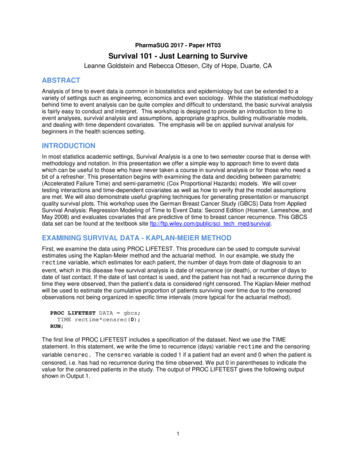
Survival 101 – Just Learning to Survive, continuedremove the grade covariate from the MODEL statement and put it into a STRATA statement. The MODELstatement then only includes nodes, hormones, and prog recp. Grade will automatically be treated ascategorical so it can also be removed from the CLASS statement.PROC PHREG DATA gbcs;CLASS nodes(REF 'N1') hormone(REF 'No') prog recp(REF 'Negative') /PARAM REF;MODEL rectime*censrec(0) hormone nodes prog recp / RL;STRATA grade;FORMAT nodes nodes. hormone ynf. prog recp posneg.;RUN;The Partial Output of the PROC PHREG stratified by grade is shown below.Output 9. Partial Output from PROC PHREG for Cox Proportional Hazards Model stratified bygradeWe compare the hazard ratios in Output 9 to those in Output 7. We expect the covariates to be somewhatdifferent in the two model outputs. We see that the covariates change using stratification, but only slightly.The choice in using stratification or including time-dependent covariates in the model depends on theimportance of the covariate that does not meet that proportional hazards assumption. If the variable isclinically important to the time to event outcome then we may prefer to use time-dependent covariatesover stratification since with the use of stratification no coefficient is provided for grade.CREATING SURVIVAL PLOTSWe’ve shown how to create a basic survival plot with the use of ODS GRAPHICS ON in the LIFETESTprocedure. These graphics are the defaults that come with the procedure and are fine for analysis butmay not be presentation or publication ready. Creating good looking survival plots is still easy to do withvarious options as well as other methods for producing graphs.There are many ways to produce graphics in SAS and the choice of which method to use depends onthe users background and the desired flexibility. The twomethods that we will cover are:1) Using ODS graphics is easy and the plots that areproduced come with the standard graphics for theappropriate analysis. The user can create editablepoint and click graphics. This method is limited in thatchanges can only be made with certain options.2) The ODS Graphics Designer tool is a click and pointinterface that makes it very easy to customizegraphics and will also save complicated templatecoding. The user need to know more about whatgraphic is appropriate for the analysis, and dependingon the analysis the statistical estimates sometimes need to be output to a data set before thegraph can be produced.Figure 1. Simple survival plot13
Survival 101 – Just Learning to Survive, continuedThere are certainly other ways to make nice graphics in SAS such as utilizing the SG procedures or usingthe Graph Template Language (GTL). However our aim is to cover simple ways to conduct survivalanalysis and make corresponding graphics so we will focus on
Survival 101 – Just Learning to Survive, continued . 4 . specify TEST LOGRANK as an option in the STRATA statement. The grade covariate has three levels. Therefore, we wish to adjust the results of the log-rank test for multiple comparisons using the ADJUST SIDAK option. The resu