Transcription
Topic 3 - Survival Analysis –1. Topics . . . . . . . . . . . . . . . . . . . . . . . . . . . . . . . . . . . . . . . . . . . . . . . . . . . 22. Learning objectives . . . . . . . . . . . . . . . . . . . . . . . . . . . . . . . . . . . . . . . . . 33. Grouped survival data - leukemia example . . . . . . . . . . . . . . . . . . . . . . 43.1 Cohort survival data schematic . . . . . . . . . . . . . . . . . . . . . . . . . 53.2 Tabulation of events and time at risk . . . . . . . . . . . . . . . . . . . . . 63.3 Stata commands for survival data . . . . . . . . . . . . . . . . . . . . . . 103.4 Displaying incidence (hazard) rates . . . . . . . . . . . . . . . . . . . . 163.5 Survivor function, S(t) . . . . . . . . . . . . . . . . . . . . . . . . . . . . . . . 173.6 Displaying survivor function, S(t) . . . . . . . . . . . . . . . . . . . . . . . 224. Stata do-file scripts: cl10ex1.do, cl10ex1a.do,cl10ex2.do . . . . . . . . . . . . . . . . . . . . . . . . . . . . . . . . . . . . . . . . . . . 244.1 AML example – cl10ex1.do . . . . . . . . . . . . . . . . . . . . . . . . . . . 255. Kaplan-Meier estimate of survivor function, S(t) . . . . . . . . . . . . . . . . . . 305.1 Kaplan-Meier estimate of survivor function, S(t) . . . . . . . . . . . 325.2 Example: Kaplan-Meier survival curves for the AML data . . . . 355.3 Confidence interval for S(t) – Greenwood’s formula . . . . . . . . 415.4 Better CI for S(t) – complementary log-log transform . . . . . . . 426. Log-rank test for comparing survivor curves . . . . . . . . . . . . . . . . . . . . 507. Stata do-file script: cl12ex1.do . . . . . . . . . . . . . . . . . . . . . . . . . . . . . . . 538. Cox proportional hazards regression model . . . . . . . . . . . . . . . . . . . . . 578.1 Regression model . . . . . . . . . . . . . . . . . . . . . . . . . . . . . . . . . . 578.2 Partial likelihood . . . . . . . . . . . . . . . . . . . . . . . . . . . . . . . . . . . 618.3 Example: Cox PH model for AML data . . . . . . . . . . . . . . . . . . 638.4 Example: Cox PH model for CABG surgery . . . . . . . . . . . . . . 668.5 Stata do-file for example . . . . . . . . . . . . . . . . . . . . . . . . . . . . . 75JHU Graduate Summer Institute of Epidemiology and Biostatistics, June 16- June 27, 2003Materials extracted from: Biostatistics 623 2002 by JHU Biostatistics Dept.Topic 3 - 1
1. Topics!Introduce survival analysis with grouped data!Estimation of the hazard rate and survivorfunction!Kaplan-Meier curves to estimate the survivalfunction, S(t)!Standard errors and 95% CI for the survivalfunction!Cox proportional hazards model! Key words: survival function, hazard, groupeddata, Kaplan-Meier, log-rank test, hazardregression, relative hazardJHU Graduate Summer Institute of Epidemiology and Biostatistics, June 16- June 27, 2003Materials extracted from: Biostatistics 623 2002 by JHU Biostatistics Dept.Topic 3 - 2
2. Learning objectives!Describe the survival time density function,survival function, and hazard function!Describe how to estimate and use the KaplanMeier survival curve and confidence intervals!Describe and use a log-rank test to comparetwo survival curves!Describe and use the Cox proportional hazardsmodel to compare survival experienceJHU Graduate Summer Institute of Epidemiology and Biostatistics, June 16- June 27, 2003Materials extracted from: Biostatistics 623 2002 by JHU Biostatistics Dept.Topic 3 - 3
3. Grouped survival data - leukemia example! Consider a clinical trial in patients with acutemyelogenous leukemia (AML) comparing twogroups of patients: no maintenance treatmentwith chemotherapy (X 0) -vs- maintenancechemotherapy treatment (X 1)GroupWeeks in remission -- ie,time to relapseMaintenance chemo(X 1)9, 13, 13 , 18, 23, 28 ,31, 34, 45 , 48, 161 No maintenance chemo 5, 5, 8, 8, 12, 16 , 23, 27,(X 0)30 , 33, 43, 45 indicates a censored time to relapse; e.g.,13 more than 13 weeks to relapseJHU Graduate Summer Institute of Epidemiology and Biostatistics, June 16- June 27, 2003Materials extracted from: Biostatistics 623 2002 by JHU Biostatistics Dept.Topic 3 - 4
3.1 Cohort survival data schematicJHU Graduate Summer Institute of Epidemiology and Biostatistics, June 16- June 27, 2003Materials extracted from: Biostatistics 623 2002 by JHU Biostatistics Dept.Topic 3 - 5
3.2 Tabulation of events and time at risk! Divide the time period into intervals appropriate forthe data– use more intervals in periods of changingincidence! For each person, tally time spent at risk (personyears) in each interval– these are the denominators for rates! Tally the events in each interval– these counts are the numerators for therates and are the values of theresponse variableJHU Graduate Summer Institute of Epidemiology and Biostatistics, June 16- June 27, 2003Materials extracted from: Biostatistics 623 2002 by JHU Biostatistics Dept.Topic 3 - 6
3.2 Tabulation of events and time at riskJHU Graduate Summer Institute of Epidemiology and Biostatistics, June 16- June 27, 2003Materials extracted from: Biostatistics 623 2002 by JHU Biostatistics Dept.Topic 3 - 7
3.2 Tabulation of events and time at risk! Divide follow-up time in the AML example into 15intervals (defined below in the table) and handtally each patient’s follow-up time in weeks toproduce the following summary table of eventsand person-timeMaintained onchemoNot maintained 335-40015010JHU Graduate Summer Institute of Epidemiology and Biostatistics, June 16- June 27, 2003Materials extracted from: Biostatistics 623 2002 by JHU Biostatistics Dept.Topic 3 - 8
3.2 Tabulation of events and time at risk40-450152845-5018--50 0111--JHU Graduate Summer Institute of Epidemiology and Biostatistics, June 16- June 27, 2003Materials extracted from: Biostatistics 623 2002 by JHU Biostatistics Dept.Topic 3 - 9
3.4 Displaying incidence (hazard) ratesStata commands for survival data! There are many Stata commands for input,management, and analysis of survival data,most of which are found in the manual in the stsection – all survival data commands start withst! st can be used to analyze individual level data(Kaplan-Meier, Cox regression, etc) or to groupthe individual level data for grouped analysis(SMRs, output for Poisson regression, etc)! Table of contents for st command, Stata 7Reference manualJHU Graduate Summer Institute of Epidemiology and Biostatistics, June 16- June 27, 2003Materials extracted from: Biostatistics 623 2002 by JHU Biostatistics Dept.Topic 3 - 10
3.4 Displaying incidence (hazard) ratesJHU Graduate Summer Institute of Epidemiology and Biostatistics, June 16- June 27, 2003Materials extracted from: Biostatistics 623 2002 by JHU Biostatistics Dept.Topic 3 - 11
3.4 Displaying incidence (hazard) rates! Outline for survival data input and analysis:With data that are already grouped intoappropriate time intervals:1.Enter the data on counts,denominators, and Xs into Stata(bypass the st commands)With ungrouped survival data on individuals:1.Use the ordinary Stata inputcommands to input and/orgenerate the following variables:X variablesDenominator variable (ifapplicable)Time variable containing followup timeCensoring variable indicatingstatus at the end of followup either “failed” or“censored”JHU Graduate Summer Institute of Epidemiology and Biostatistics, June 16- June 27, 2003Materials extracted from: Biostatistics 623 2002 by JHU Biostatistics Dept.Topic 3 - 12
3.4 Displaying incidence (hazard) rates2.Then, use the st commands, asillustrated below, below toprocess and analyze the data! Define survival data:stset commandUsed to define the time variable, the statusvariable with the codes for “failures,” andan “Id” variable the uniquely identifies eachindividual observationstset t , failure(failed 1) id(id)! Descriptive statistics for survival data:stdes, stsum commandJHU Graduate Summer Institute of Epidemiology and Biostatistics, June 16- June 27, 2003Materials extracted from: Biostatistics 623 2002 by JHU Biostatistics Dept.Topic 3 - 13
3.4 Displaying incidence (hazard) rates. stdes if x 0failure d:analysis time t:id:failed 1tid -------------- per subject -------------- ------no. of subjects12no. of records121111(first) entry time(final) exit timesubjects with gaptime on gap if gaptime at ---------------------------------------. stdes if x 1ETC. stsum , by(x)failure d:analysis time t:id:failed 1tid incidenceno. of ------ Survival time ----- x time at riskratesubjects25%50%75%--------- ------------------1 423.0165485111831480 255.03921571282343--------- ------------------total 678.025073723122743JHU Graduate Summer Institute of Epidemiology and Biostatistics, June 16- June 27, 2003Materials extracted from: Biostatistics 623 2002 by JHU Biostatistics Dept.Topic 3 - 14
3.4 Displaying incidence (hazard) rates!Compare overall incidence by groups:stir command. stir xfailure d:analysis time t:id:note:failed 1tidExposed - x 1 and Unexposed - x 0 x ExposedUnexposed Total----------------- ------------------------ ---------Failure 107 17Time 255423 678----------------- ------------------------ --------- Incidence Rate .0392157.0165485 .0250737 Point estimate [95% Conf. Interval] ------------------------ ---------------------Inc. rate diff. .0226672 -.004555.0498895Inc. rate ratio 2.369748 .81419347.334788Attr. frac. ex. .5780142 -.2282095.8636634Attr. frac. pop .3400083 p)Pr(k 10) 0.0418(midp) 2*Pr(k 10) 0.0836!(exact)(exact)(exact)(exact)Bin the time for grouped survival analysis:stsplit command* Specify ends of intervals, last interval extends toinfinitystsplit tbin , at( 2.5(2.5)20,!25, 30, 35, 40, 45, 50, 161 )Tabulate rates by a categorical variable group(x) and bins (groups) offollow-up time:strate command* Output to new dataset: D eventsY time at riskRate ratestrate tbin x , output(binrates.dta,replace)JHU Graduate Summer Institute of Epidemiology and Biostatistics, June 16- June 27, 2003Materials extracted from: Biostatistics 623 2002 by JHU Biostatistics Dept.Topic 3 - 15
3.4 Displaying incidence (hazard) rates!Incidence rates -- also called hazard ratessimply estimated as the ratio of the number ofevents to the total time at risk in an interval: !To display the incidence rates:— Plotlog incidence -vs- timestratified by groups of interest( plotting incidence -vs- time on a semi- logscale has the same effect andpreserves the original units for therates)— Plots are especially useful when the persontime denominators are large in each group;ie, when the estimates are not too noisyJHU Graduate Summer Institute of Epidemiology and Biostatistics, June 16- June 27, 2003Materials extracted from: Biostatistics 623 2002 by JHU Biostatistics Dept.Topic 3 - 16
3.6 Displaying survivor function, S(t)!The “Survivor Function” is defined asS(t) Pr (Survived beyond time t)! For example,suppose t end of follow-up timebin 3S(t) Pr (Survived t) Pr (survived through bin 1 andsurvived through bin 2 andsurvived through bin 3) !Pr(survived bin 1) xPr(survived bin 2 given survived bin 1) xPr(survived bin 3 given survived bin 1 andbin 2)Calculate probabilities of surviving through bin j offollow-up time by finding the complement of theprobability of dying in bin jJHU Graduate Summer Institute of Epidemiology and Biostatistics, June 16- June 27, 2003Materials extracted from: Biostatistics 623 2002 by JHU Biostatistics Dept.Topic 3 - 17
3.6 Displaying survivor function, S(t)Pr (Survived bin j) 1 - Pr(died in bin j)! Pr ( “Die” in bin j ) is approximated byPj Pj whereyj # of events in bin jNj time at risk (person-time) in bin jLj length of bin j (must be small for theapproximation to workwell)JHU Graduate Summer Institute of Epidemiology and Biostatistics, June 16- June 27, 2003Materials extracted from: Biostatistics 623 2002 by JHU Biostatistics Dept.Topic 3 - 18
3.6 Displaying survivor function, S(t)!Then, use Pj , the probabilities of dying in bin j, toestimate the survivor function, S(t):(t) [ 1 - Pr(Die in j) ] ( 1 - Pj ).! The calculations needed for(t), the estimatedsurvivor function, are usually organized into a“life table, as follows:Sj Pr ( Survived beyond the end of bin j)S0 1JHU Graduate Summer Institute of Epidemiology and Biostatistics, June 16- June 27, 2003Materials extracted from: Biostatistics 623 2002 by JHU Biostatistics Dept.Topic 3 - 19
3.6 Displaying survivor function, S(t)Maintained on chemojLjNjyj12.527.522.53Not maintained on chemo1-Pj SjNjyj1-Pj 61351501.291820*014581.375.109-01511111101.109-01- yi Lj/Nj1-yi Lj/Nj.553JHU Graduate Summer Institute of Epidemiology and Biostatistics, June 16- June 27, 2003Materials extracted from: Biostatistics 623 2002 by JHU Biostatistics Dept.Topic 3 - 20
3.6 Displaying survivor function, S(t)!Trouble with follow-up time bins that are too wide:1-Pj 1-yi Lj /Nj 1-(10/8) -0.25Work-around: set the probability, 1 - Pj , to zerowhenever the estimate isnegativeJHU Graduate Summer Institute of Epidemiology and Biostatistics, June 16- June 27, 2003Materials extracted from: Biostatistics 623 2002 by JHU Biostatistics Dept.Topic 3 - 21
3.6 Displaying survivor function, S(t)!To display the estimated survivor,plot(t) -vs- t— For grouped data:Plot(t) at the end of each time intervalconnecting the points with linesegments (not steps like KaplanMeier)At time 0, plot(t)/1JHU Graduate Summer Institute of Epidemiology and Biostatistics, June 16- June 27, 2003Materials extracted from: Biostatistics 623 2002 by JHU Biostatistics Dept.Topic 3 - 22
3.6 Displaying survivor function, S(t)JHU Graduate Summer Institute of Epidemiology and Biostatistics, June 16- June 27, 2003Materials extracted from: Biostatistics 623 2002 by JHU Biostatistics Dept.Topic 3 - 23
4. Stata do-file scripts: cl10ex1.do, cl10ex1a.do,cl10ex2.do!The Stata script for the AML data example,including commands for inputting survival dataand grouping the survival data on the courseweb site:cl10ex1.do(The raw data are contained in the script)!Another related script for the AML data shows howto input the grouped survival data directly intoStata as you might had you tabulated thegrouped data by hand:cl10exa.doJHU Graduate Summer Institute of Epidemiology and Biostatistics, June 16- June 27, 2003Materials extracted from: Biostatistics 623 2002 by JHU Biostatistics Dept.Topic 3 - 24
4.1 AML example – cl10ex1.doversion 7.0*CL10EX1.DOGrouped survival data***AML data:weeks in remission -vs-*Raw data:AML data included below* Assumes files are in folder**treatment group[path]\bio623If files are in another folder, change cdpoint Stata to the correct folder* To run this program,command below touse the following Stata commands:*cd [path]\bio623*do. change directory to folder bio623cl10ex1* tPartPartParta.b.c.d.e.f.g.h.i.j.k.Input data, define as a survival datasetDefine survival variables: stsetDescriptive summaries: stdes, stsumBin the time for grouped survival analysis: stsplitTabulate rates by categorical variable group(x) and bins: strateCalculate survivor function, S(t) from grouped dataPlot Survivor function S(t) for grouped dataFit different log-linear models for group(x) , get deviances and AICPlot estimated hazard functions for models A-EFit non-proportional hazard for group effect -- Model FUse Model D to estimate and plot smoothed S(t)* Housekeeping* Clear workspaceJHU Graduate Summer Institute of Epidemiology and Biostatistics, June 16- June 27, 2003Materials extracted from: Biostatistics 623 2002 by JHU Biostatistics Dept.Topic 3 - 25
clear* Turn off -more- pauseset more off* Save log file on disk, use .log so Notepad will open itcapture log closelog using cl10ex1.log, replace* Make subfolder for graphsshell md cl10ex1* Extend linesize for logset log linesize 100* Part a.*id,Input data, define as a survival datasetx(0 no maint 1 maint), t time to relapse,input id x11 921 1331 1341 1851 2361 2871 3181 3491 4510 1 4811 1 16112 0 513 0 514 0 815 0 816 0 1217 0 1618 0 2319 0 2720 0 3021 0 3322 0 4323 0 45endfailed (1 relaspsed 0 censored)t failed00100100101000001001000JHU Graduate Summer Institute of Epidemiology and Biostatistics, June 16- June 27, 2003Materials extracted from: Biostatistics 623 2002 by JHU Biostatistics Dept.Topic 3 - 26
* Part b.Define survival variables:stsetstset t , failure(failed 1) id(id)* Save as Stata datasetsave cl10ex1.dta , replace* Part c.Descriptive summaries:stdes, stsum* Simple counts of persons, events, time at riskstdes if x 1stdes if x 0* Summary stats:time at risk, rates, subject, 25,50,75 %tiles (K-M estimates)stsum , by(x)* Compare overall incidence rates by group:stirstir x* Part d.Bin the time for grouped survival analysis:*Expands dataset, 1 record for each person-time interval combinationNote:stsplit* Specify ends of intervals, last interval extends to infinitystsplit tbin , at( 2.5 (2.5) 20, 25,30,35,40,45,50,161 )* Part e.** NOTE:Tabulate rates by categorical variable group(x) and bins:Output to new dataset: D eventsThe strate commandY time at riskstrateRate rateREQUIRES STATA 6 or 7strate tbin x , output(binrates.dta,replace)JHU Graduate Summer Institute of Epidemiology and Biostatistics, June 16- June 27, 2003Materials extracted from: Biostatistics 623 2002 by JHU Biostatistics Dept.Topic 3 - 27
* Part f.Calculate survivor function, S(t)from grouped data* Access rates, time at risk datasetuse binrates.dta , clear* UGH:For some reason, Y was created as a string!!Convert to numericgen temp real( Y)drop Ygen Y tempdrop temp* First, calculate interval lengths, L, for grouped survival analysis* Make sure in order by group(x) and time binsort x tbin*L subtract lower limtits for interval n 1 -vs- n ; last( N) interval isundefinedby x:gen L cond( n N , tbin[ n 1] - tbin , . )* Calculate midpoints f intevals for log-linear models -- last intervals must be*treated as special casesgen midT tbin L/2replace midT 42.5 if(x 1 & midT .)replace midT 105.5 if (x 0 & midT .)* Calculate survival probs P for each interval: rate x length, (correct if P 0)gen P min(1 - Rate*L,1)* Calculate S(t) Prob (Surviving beyond t) Product P1 P2 . Ptgen S Pby x: replace S cond( n 1, P*S[ n-1] , S)* Show results Y time at riskD failureslist midT x Y D P S* Part g.Plot Survivor function S(t) for grouped dataJHU Graduate Summer Institute of Epidemiology and Biostatistics, June 16- June 27, 2003Materials extracted from: Biostatistics 623 2002 by JHU Biostatistics Dept.Topic 3 - 28
*Plot S(t) for grouped data at end of intervals; connect with lines* To plot S(t) for each of two groups, need two variables* Plot S(t) at end of interval lower limit length/2 , last interval not used*by convention, plot S(0) 1gen T tbinby x: gen MAINT cond( n 1, S[ n-1], 1)if x 1by x: gen NOMAINT cond( n 1, S[ n-1], 1)if x 0* Check shifted plotting points*list tbin L T S MAINT NOMAINTset textsize 140#delimit ;graph MAINT NOMAINT T , symbol(OS) connect(ll) xlab ylabl1(" ") l2("S(t) PROBABILITY RELAPSE t ")b1(" ") b2("WEEKS")t2("Survivor Function for Binned AML Data");#delimit cr;gphprint , saving(cl10ex1\figg1.wmf,replace)drop T P S MAINT NOMAINT* Close log file -- Only when all errors have been fixed*log closeJHU Graduate Summer Institute of Epidemiology and Biostatistics, June 16- June 27, 2003Materials extracted from: Biostatistics 623 2002 by JHU Biostatistics Dept.Topic 3 - 29
5.Kaplan-Meier estimate of survivor function, S(t)Paul Meier was an assistant professor in theJHU Department of Biostatistics from 1952 to1957. He teamed with E.L. Kaplan to write theirseminal paper "Non-parametric Estimation fromIncomplete Observations," which appeared inthe Journal of the American StatisticalAssociation in 1958. This paper was to lay thegroundwork for modern survival analysis. Herecently retired as chair of the Department ofStatistics at Columbia University, where hemade important contributions to the methods forand practice of clinical trials.JHU Graduate Summer Institute of Epidemiology and Biostatistics, June 16- June 27, 2003Materials extracted from: Biostatistics 623 2002 by JHU Biostatistics Dept.Topic 3 - 30
! In the “not maintained on chemotherapy” group:times of events/censoringtime(t)16 # atrisk#eventsfraction ofeventsfraction noeventsfractionsurviving after 0040014/681100422/42/44/6 x 2/4 2/690020012/6100020012/6110020012/6121021½½2/6 x ½ 1/613010111/614010111/615010111/616010111/6!!JHU Graduate Summer Institute of Epidemiology and Biostatistics, June 16- June 27, 2003Materials extracted from: Biostatistics 623 2002 by JHU Biostatistics Dept.Topic 3 - 31
5.1 Kaplan-Meier estimate of the survivor function,S(t)! For grouped survival data, Estimated Pr (Survive beyond t)(*) ! Let interval lengths Lj become very small - all oflength L )t and let t1, t2, . be times of events(survival times)! 2 cases to consider in (*)Case 1. No event in bin (interval) Y1- 0 1(t) does not change - which means thatwe can ignore bins with no eventsJHU Graduate Summer Institute of Epidemiology and Biostatistics, June 16- June 27, 2003Materials extracted from: Biostatistics 623 2002 by JHU Biostatistics Dept.Topic 3 - 32
5.1 Kaplan-Meier estimate of the survivor function,S(t)Case 2. yj events occur in a bin (interval)Also:nj persons enter the binassume any censored timesthat occur in the binoccur at the end ofthe bin1- 1- JHU Graduate Summer Institute of Epidemiology and Biostatistics, June 16- June 27, 2003Materials extracted from: Biostatistics 623 2002 by JHU Biostatistics Dept.Topic 3 - 33
5.1 Kaplan-Meier estimate of the survivor function,S(t)! So, as )t 6 0, we get the Kaplan- Meier estimateof the survivor function, S(t):(t) (IMPORTANT)(0) / 1 (by convention)Also called the “product-limit estimate” ofthe survivor function, S(t)JHU Graduate Summer Institute of Epidemiology and Biostatistics, June 16- June 27, 2003Materials extracted from: Biostatistics 623 2002 by JHU Biostatistics Dept.Topic 3 - 34
5.2 Example: Kaplan-Meier survival curves forthe AML data! Calculation of Kaplan-Meier estimates:In the “not maintained on chemotherapy” group:TimeAt riskEvents(t)tjnjyj(tj) 01201.051221.0 x ((12-2)/2) 0.83381020.833 x ((102)/10) 0.66612810.666 x ((8-1)/8) 0.58323610.583 x ((6-1)/6) 0.48627510.486 x ((5-1)/5) 0.38933310.389 x ((3-1)/3) 0.25943210.259 x ((2-1)/2) 0.13045110.130 x ((1-1)/1) 0JHU Graduate Summer Institute of Epidemiology and Biostatistics, June 16- June 27, 2003Materials extracted from: Biostatistics 623 2002 by JHU Biostatistics Dept.Topic 3 - 35
5.2 Example: Kaplan-Meier survival curves forthe AML dataIn the “maintained on chemotherapy” group:TimeAt riskEvents(t)tjnjyj(tj) 01101.09111.909 13101.818 1881.7162371.6143151.4913441.3684821.184JHU Graduate Summer Institute of Epidemiology and Biostatistics, June 16- June 27, 2003Materials extracted from: Biostatistics 623 2002 by JHU Biostatistics Dept.Topic 3 - 36
5.2 Example: Kaplan-Meier survival curves forthe AML data! The “Kaplan-Meier curve” plots the estimatedsurvival function (t) -vs- time -- separatecurves for each groupJHU Graduate Summer Institute of Epidemiology and Biostatistics, June 16- June 27, 2003Materials extracted from: Biostatistics 623 2002 by JHU Biostatistics Dept.Topic 3 - 37
5.2 Example: Kaplan-Meier survival curves forthe AML data! Notes— Can count the total number of events bycounting the number of steps (times)— If feasible, picture the censoring times on thegraph as shown above! Stata code for Kaplan-Meier estimates and plots— Input data and define as a survival datasetJHU Graduate Summer Institute of Epidemiology and Biostatistics, June 16- June 27, 2003Materials extracted from: Biostatistics 623 2002 by JHU Biostatistics Dept.Topic 3 - 38
5.2 Example: Kaplan-Meier survival curves forthe AML data* Raw data: id, x(0 no maint 1 maint),t time to relapse,failed (1 relapsed 0 censored)input id x t failed1 1 9 12 1 13 13 1 13 0þend* Define survival variables: stsetstset t , failure(failed 1) id(id)— Calculate and print Kaplan-Meier estimatesfor each groupsts list if x 1sts list if x 0Stata log:. sts listif x 1failure d:analysis time t:failed 1tJHU Graduate Summer Institute of Epidemiology and Biostatistics, June 16- June 27, 2003Materials extracted from: Biostatistics 623 2002 by JHU Biostatistics Dept.Topic 3 - 39
5.2 Example: Kaplan-Meier survival curves forthe AML ionError[95% Conf. ----— Plot Kaplan-Meier curves; list counts ofcensored on plots* Plot Kaplan-Meier estimatessts graph , by(x) lost( Graph shown above)JHU Graduate Summer Institute of Epidemiology and Biostatistics, June 16- June 27, 2003Materials extracted from: Biostatistics 623 2002 by JHU Biostatistics Dept.Topic 3 - 40
5.3 Confidence interval for S(t) -- Greenwood’sformula! Greenwood’s formula for the variance of (t):[(t) ] (t)2SEGW(t) ! Using Greenwood’s formula, an approximate 95%CI for S(t) is(t) 2 SEGW(t)! There is a “problem”: the 95% CI is notconstrained to lie within the interval (0,1)JHU Graduate Summer Institute of Epidemiology and Biostatistics, June 16- June 27, 2003Materials extracted from: Biostatistics 623 2002 by JHU Biostatistics Dept.Topic 3 - 41
5.4 Better CI for S(t) -- complementary log-logtransform! Consider the “Complementary log log transform”(CLL):(t) log [ - log(t)]JHU Graduate Summer Institute of Epidemiology and Biostatistics, June 16- June 27, 2003Materials extracted from: Biostatistics 623 2002 by JHU Biostatistics Dept.Topic 3 - 42
5.4 Better CI for S(t) -- complementary log-logtransform! Variance of CLL:(t) log [-log((t) )(t)] SECLL(t) JHU Graduate Summer Institute of Epidemiology and Biostatistics, June 16- June 27, 2003Materials extracted from: Biostatistics 623 2002 by JHU Biostatistics Dept.Topic 3 - 43
5.4 Better CI for S(t) -- complementary log-logtransform! Use CLL to obtain 95% CI on S(t)1. Get 95% CI for v(t):(t) 2 SECLL(t)2. Transform back to get 95% CI for S(t):Use the inverse transformationS(t) to get the 95% CI for S(t):[,] ( NOTE: Stata uses the CLL transformation for95% CI on S(t) -- see log above)! Example: Back to the AML dataJHU Graduate Summer Institute of Epidemiology and Biostatistics, June 16- June 27, 2003Materials extracted from: Biostatistics 623 2002 by JHU Biostatistics Dept.Topic 3 - 44
5.4 Better CI for S(t) -- complementary log-logtransform!TimeAt 143151.4913441.3684821.184(13)]Greenwood [ .8182 ( ) (.116)2! 95% CIGreenwood .818 2 (.116) (.586, 1.05)1.05 is out of rangeJHU Graduate Summer Institute of Epidemiology and Biostatistics, June 16- June 27, 2003Materials extracted from: Biostatistics 623 2002 by JHU Biostatistics Dept.Topic 3 - 45
5.4 Better CI for S(t) -- complementary log-logtransform! Better 95% CI using the CLL transformation:(t) log(-log((13) (t)) -1.605 .502SECLL (13) .708! 95% CI for S(13) (.437, .952)JHU Graduate Summer Institute of Epidemiology and Biostatistics, June 16- June 27, 2003Materials extracted from: Biostatistics 623 2002 by JHU Biostatistics Dept.Topic 3 - 46
5.4 Better CI for S(t) -- complementary log-logtransform! 95% CI for S(t) in the maintained onchemotherapy groupTimeAt risk Events(t)95% 3441.37.163.09,.654821.18.154 .01,.53*Based on complementary log-log transformJHU Graduate Summer Institute of Epidemiology and Biostatistics, June 16- June 27, 2003Materials extracted from: Biostatistics 623 2002 by JHU Biostatistics Dept.Topic 3 - 47
5.4 Better CI for S(t) -- complementary log-logtransform! 95% CI for S(t) in the not maintained onchemotherapy groupTimeAt risk Events(t)95% 6.14.05,.554321.13.12.01,.424511.00*Based on complementary log-log transform-JHU Graduate Summer Institute of Epidemiology and Biostatistics, June 16- June 27, 2003Materials extracted from: Biostatistics 623 2002 by JHU Biostatistics Dept.Topic 3 - 48
5.4 Better CI for S(t) -- complementary log-logtransformJHU Graduate Summer Institute of Epidemiology and Biostatistics, June 16- June 27, 2003Materials extracted from: Biostatistics 623 2002 by JHU Biostatistics Dept.Topic 3 - 49
6. Log-rank test for c
Jun 27, 2003 · Introduce survival analysis with grouped data! Estimation of the hazard rate and survivor function! Kaplan-Meier curves to estimate the survival function, S(t)! Standard errors and 95% CI for the survival function! Cox proportional hazards model! Key words: survival function, hazard, grouped