Transcription
Inverse Decision Modeling:Learning Interpretable Representations of BehaviorDaniel Jarrett 1 * Alihan Hüyük 1 * Mihaela van der Schaar 1 2AbstractConsider the “lifecycle” of decision analysis [9] in the realworld. First, normative analysis deals with modeling rational decision-making. It asks the question: What constitutesideal behavior? To this end, a prevailing approach is givenby von Neumann-Morgenstern’s expected utility theory, andthe study of optimal control is its incarnation in sequentialdecision-making [10]. But judgment rendered by real-worldagents is often imperfect, so prescriptive analysis deals withimproving existing decision behavior. It asks the question:How can we move closer toward the ideal? To this end, thestudy of decision engineering seeks to design “human-in-theloop” techniques that nudge or assist decision-makers, suchas medical guidelines and best practices [11]. Importantly,however, this first requires a quantitative account of currentpractices and the imperfections that necessitate correcting.Decision analysis deals with modeling and enhancing decision processes. A principal challenge inimproving behavior is in obtaining a transparentdescription of existing behavior in the first place.In this paper, we develop an expressive, unifyingperspective on inverse decision modeling: a framework for learning parameterized representationsof sequential decision behavior. First, we formalize the forward problem (as a normative standard),subsuming common classes of control behavior.Second, we use this to formalize the inverse problem (as a descriptive model), generalizing existingwork on imitation/reward learning—while opening up a much broader class of research problemsin behavior representation. Finally, we instantiatethis approach with an example (inverse boundedrational control), illustrating how this structureenables learning (interpretable) representations of(bounded) rationality—while naturally capturingintuitive notions of suboptimal actions, biased beliefs, and imperfect knowledge of environments.To take this crucial first step, we must therefore start withdescriptive analysis—that is, with understanding observeddecision-making from demonstration. We ask the question:What does existing behavior look like—relative to the ideal?Most existing work on imitation learning (i.e. to replicate expert actions) [12] and apprenticeship learning (i.e. to matchexpert returns) [13] offers limited help, as our objective is instead in understanding (i.e. to interpret imperfect behavior).In particular, beyond the utility-driven nature of rationalityfor agent behaviors, we wish to quantify intuitive notions ofboundedness—such as the apparent flexibility of decisions,tolerance for surprise, or optimism in beliefs. At the sametime, we wish that such representations be interpretable—that is, that they be projections of observed behaviors ontoparameterized spaces that are meaningful and parsimonious.1. IntroductionModeling and enhancing decision-making behavior is a fundamental concern in computational and behavioral science,with real-world applications to healthcare [1], economics [2],and cognition [3]. A principal challenge in improving decision processes is in obtaining a transparent understanding ofexisting behavior to begin with. In this pursuit, a key complication is that agents are often boundedly rational due tobiological, psychological, and computational factors [4–8],the precise mechanics of which are seldom known. As such,how can we intelligibly characterize imperfect behavior?1Department of Applied Mathematics and Theoretical Physics, University of Cambridge, UK; 2 Department of Electrical Engineering,University of California, Los Angeles, USA. Authors contributedequally. Correspondence to: daniel.jarrett@maths.cam.ac.uk .Proceedings of the 38 th International Conference on MachineLearning, PMLR 139, 2021. Copyright 2021 by the author(s).Contributions In this paper, our mission is to explicitlyrelax normative assumptions of optimality when modelingdecision behavior from observations.3 First, we develop anexpressive, unifying perspective on inverse decision modeling: a general framework for learning parameterized representations of sequential decision-making behavior. Specifically, we begin by formalizing the forward problem F (as3Our terminology is borrowed from economics: By “descriptive”models, we refer to those that capture observable decision-makingbehavior as-is (e.g. an imitator policy in behavioral cloning), andby “normative” models, we refer to those that specify optimal decision-making behavior (e.g. with respect to some utility function).
Inverse Decision ModelingTable 1. Inverse Decision Modeling. Comparison of primary classes of imitation/ reward learning (IL/IRL) versus our prototypicalexample (i.e. inverse bounded rational control) as instantiations ofinverse decision modeling. Constraints on agent behavior include:†environment dynamics (extrinsic), and ‡ bounded rationality (intrinsic). Legend: deterministic (Det.), stochastic (Stoc.), subjectivedynamics (Subj.), behavioral cloning (BC), distribution matching(DM), risk-sensitive (RS), partially-observable (PO), maximumentropy (ME). All terms/notation are developed over Sections 3–4. env iorPartiallyObservableInverseDecision ModelPartiallyControllableExtrinsic†Examples ,! , BC-ILSubj. BC-IL333377733377777777 [14–21][22]Det. DM-ILStoc. DM-IL337777777377777777[23, 24][25–39]Det. IRLStoc. IRLSubj. �46][47–66][67][68, 69]Det. PO-IRLStoc. PO-IRLSubj. ][77–80]ME-IRLSubj. ME-IRL337733733377337777[81–92][93, 94]Inverse BoundedRational Control 333333333 Section 4a normative standard), showing that this subsumes common classes of control behavior in literature. Second, weuse this to formalize the inverse problem G (as a descriptive model), showing that it generalizes existing work onimitation and reward learning. Importantly, this opens upa much broader variety of research problems in behaviorrepresentation learning—beyond simply learning optimalutility functions. Finally, we instantiate this approach withan example that we term inverse bounded rational control, illustrating how this structure enables learning (interpretable)representations of (bounded) rationality—capturing familiarnotions of decision complexity, subjectivity, and uncertainty.2. Related WorkAs specific forms of descriptive modeling, imitation learning and apprenticeship learning are popular paradigms forlearning policies that mimic the behavior of a demonstrator.Imitation learning focuses on replicating an expert’s actions.Classically, “behavioral cloning” methods directly seek tolearn a mapping from input states to output actions [14–16],using assistance from interactive experts or auxiliary regularization to improve generalization [17–21]. More recently,“distribution-matching” methods have been proposed forlearning an imitator policy whose induced state-action occupancy measure is close to that of the demonstrator [23–39].Apprenticeship learning focuses on matching the cumulativereturns of the expert—on the basis of some ground-truth re-ward function not known to the imitator policy. This is mostpopularly approached by inverse reinforcement learning(IRL), which seeks to infer the reward function for whichthe demonstrated behavior appears most optimal, and usingwhich an apprentice policy may itself be optimized via reinforcement learning. This includes maximum-margin methods based on feature expectations [13, 40–45], maximumlikelihood soft policy matching [51, 52], maximum entropypolicies [50, 89–92], and Bayesian maximum a posteriori inference [59–63], as well as methods that leverage preferencemodels and additional annotations for assistance [95–99].We defer to surveys of [12,100] for more detailed overviewsof imitation learning and inverse reinforcement learning.Inverse decision modeling subsumes most of the standardapproaches to imitation and apprenticeship learning as specific instantiations, as we shall see (cf. Table 1). Yet—withvery few exceptions [78–80]—the vast majority of theseworks are limited to cases where demonstrators are assumedto be ideal or close to ideal. Inference is therefore limitedto that of a single utility function; after all, its primary purpose is less for introspection than simply as a mathematicalintermediary for mimicking the demonstrator’s exhibitedbehavior. To the contrary, we seek to inspect and understandthe demonstrator’s behavior, rather than simply producing afaithful copy of it. In this sense, the novelty of our work istwo-fold. First, we shall formally define “inverse decisionmodels” much more generally as projections in the spaceof behaviors. These projections depend on our consciouschoices for forward and inverse planners, and the explicitstructure we choose for their parameterizations allows asking new classes of targeted research questions based onnormative factors (which we impose) and descriptive factors (which we learn). Second, we shall model an agent’sbehavior as induced by both a recognition policy (committing observations to internal states) and a decision policy(emitting actions from internal states). Importantly, not onlymay an agent’s mapping from internal states into actionsbe suboptimal (viz. the latter), but that their mapping fromobservations into beliefs may also be subjective (viz. the former). This greatly generalizes the idea of “boundedness” insequential decision-making—that is, instead of commonlyassumed forms of noisy optimality, we arrive at precisenotions of subjective dynamics and biased belief-updates.Appendix A gives a more detailed treatment of related work.3. Inverse Decision ModelingFirst, we describe our formalism for planners (Section 3.1)and inverse planners (Section 3.2)—together constitutingour framework for inverse decision modeling (Section 3.3).Next, we instantiate this with a prototypical example to spotlight the wider class of research questions that this unifiedperspective opens up (Section 4). Table 1 summarizes related work subsumed, and contextualizes our later example.
Inverse Decision ModelingTable 2. Planners. Formulation of primary classes of planner algorithms in terms of our (forward) formalism, incl. the boundedly rationalplanner in our example (Section 4). Legend: controlled Markov process (CMP); Markov decision process (MDP); input-output hiddenMarkov model (IOHMM); partially-observable (PO); Dirac delta ( ); any mapping into policies (f ); decision-rule parameterization ( ).Planner (F )Setting ( )Parameter ( )Decision-Rule CMP PolicyModel-Free MDP LearnerMax. Entropy MDP LearnerModel-Based MDP PlannerDifferentiable MDP PlannerKL-Regularized MDP PlannerDecision-Rule IOHMM PolicyModel-Free POMDP LearnerModel-Based POMDP PlannerBelief-Aware -POMDP PlannerS, U, TS, U, TS, U, TS, U, TS, U, TS, U, TS, X , Z, U, T , OS, X , Z, U, T , OS, X , Z, U, T , OS, X , Z, U, T , O,, , , , , , , , , , , , !,, , , !, , !Z,Bounded Rational ControlS, X , Z, U, T , O, , , , , , , %̃General FormulationS, X , Z, U, T , O(any)3.1. Forward ProblemConsider the standard setup for sequential decision-making,where an agent interacts with a (potentially partially-obser.vable) environment. First, let (S, X , Z, U , T , O) givethe problem setting, where S denotes the space of (external)environment states, X of environment observables, Z of.(internal) agent states, U of agent actions, T (S)S U of.U Senvironment transitions, and O (X )of environmentemissions. Second, denote with the planning parameter:the parameterization of (subjective) factors that a planningalgorithm uses to produce behavior, e.g. utility functions2 RS U, discount factors 2 [0, 1), or any other biases thatan agent might be subject to, such as imperfect knowledge , ! of true environment dynamics env , !env 2 T O. Notethat access to the true dynamics is only (indirectly) possiblevia such knowledge, or by sampling online/from batch data.Now, a planner is a mapping producing observable behavior:Definition 1 (Behavior) Denote the space of (observation.taction) trajectories with H [1t 0 (X U ) X . Then abehavior manifests as a distribution over trajectories (induced by an agent’s policies interacting with the environment):. (H)(1)Consider behaviors induced by an agent operating under arecognition policy 2 (Z)Z U X (i.e. committing observation-action trajectories to internal states), together witha decision policy 2 (U )Z (i.e. emitting actions frominternal states). We shall denote behaviors induced by , :.(2) , (x0 , u0 , .) P u (· z) h (x0 , u0 , .)s0 env (· s,u)x0 !env (· u,s0 )z 0 (· z,u,x0 )(Note: Our notation may not be immediately familiar aswe seek to unify terminology across multiple fields. Forreference, a summary of notation is provided in Appendix E).Optimization ( , )Examplesargmax ( fdecision ( ))[14]Pargmax E , env [ t t (st , ut )](anyRLagent)Pargmax E , env [ t t (st , ut ) H( (· st ))][101–104]Pargmax E , [ t t (st , ut )](any MDP solver)argmax ( neural-network( , , , ))[105, 106]Pargmax E , [ t t ( (st , ut ) DKL ( (· st )k ))][107–111]argmax ( fdecision ( ), frecognition ( , !))[22]Pargmax , 2{ is black-box} E , env , [ t t (st , ut )][112–117]Pargmax , 2{ is unbiased} E , , [ t t (st , ut )][118–121]P targmax , 2{ is unbiased} E , , [ t[122, 123]Z (st , zt , ut )]P targmax , 2{ is possibly-biased} E , [ t(st , ut )]Theorems 4–5 I , [ ; ]I , [ ; ] I , [%; %̃]argmax , F ( , ; )Section 3.1Definition 2 (Planner) Given problem setting and planning parameter , a planner is a mapping into behaviors:F : !(3)where indicates the space of settings, and the space ofparameters. Often, behaviors of the form , can be naturally expressed in terms of the solution to an optimization:.F ( , ) , .: , argmax , F ( , ; )(4)of some real-valued function F (e.g. this includes all caseswhere a utility function is an element of ). So, we shall.write , to indicate the behavior produced by F .This definition is very general: It encapsulates a wide rangeof standard algorithms in the literature (see Table 2), including decision-rule policies and neural-network planners.Importantly, however, observe that in most contexts, a globaloptimizer for is (trivially) either an identity function, orperfect Bayesian inference (with the practical caveat, ofcourse, that in model-free contexts actually reaching suchan optimum may be difficult, such as with a deep recurrentnetwork). Therefore in addition to just , what Definition 2makes explicit is the potential for to be biased—that is, todeviate from (perfect) Bayes updates; this will be one of theimportant developments made in our subsequent example.Note that by equating a planner with such a mapping, we areimplicitly assuming that the embedded optimization (Equation 4) is well-defined—that is, that there exists a singleglobal optimum. In general if the optimization is non-trivial,this requires that the spaces of policies , 2 P R besuitably restricted: This is satisfied by the usual (hard-/soft-Q) Boltzmann-rationality for decision policies, and byuniquely fixing the semantics of internal states as (subjective) beliefs, i.e. probability distributions over states, withrecognition policies being (possibly-biased) Bayes updates.
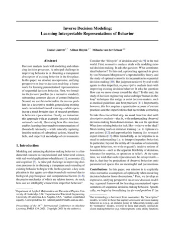
Inverse Decision ModelingFigure 1. Forward, Inverse, and Projection Mappings. In the forward direction (i.e. generation): Given planning parameters , aplanner F generates observable behavior (Definition 2). In theopposite direction (i.e. inference): Given observed behavior , aninverse planner G infers the planning parameters that producedit—subject to normative specifications (Definition 3). Finally,given observed behavior , the composition of F and G gives itsprojection onto the space of behaviors that are parameterizable by (Definition 4): This is the inverse decision model (Definition DecisionPolicy On the other extreme, the vast literature on IRL has largelyrestricted attention to perfectly optimal agents—that is, withfull visibility of states, certain knowledge of dynamics, andperfect ability to optimize . While this indeed fends off theimpossibility result, it is overly restrictive for understandingbehavior: Summarizing demo using alone is not informative as to specific types of biases we may be interested in.How aggressive does this clinician seem? How flexible dotheir actions appear? It is difficult to tease out such nuancesfrom just —let alone comparing between agents ironmentTransitionu envGeneratedBehaviorExternalStatesWe take a generalized approach to allow any middle groundof choice. While some normative specifications are requiredto fend off the impossibility result [106, 136], they need notbe so strong as to restrict us to perfect optimality. Formally:.Definition 3 (Inverse Planner) Let norm desc decompose the parameter space into a normative component(i.e. whose values norm 2 norm we wish to clamp), and adescriptive component (i.e. whose values desc 2 desc wewish to infer). Then an inverse planner is given as follows:argmax , F ( , ; )InternalStatesPlanningParameterz RecognitionPolicyargmin desc G ( , senvimit )EnvironmentResponsesEnvironmentEmissionx!envA more practical question is whether this optimum is reachable. While this may seem more difficult (at least in the mostgeneral case), for our interpretative purposes it is rarely aproblem, because (simple) human-understandable modelsare what we desire to be working with in the first instance.In healthcare, for example, diseases are often modeled interms of discrete states, and subjective beliefs over thosestates are eminently transparent factors that medical practitioners can readily comprehend and reason about [124, 125].This is prevalent in research and practice, e.g. two-to-fourstates in progressive dementia [126–128], cancer screening [129, 130], cystic fibrosis [131], as well as pulmonarydisease [132]. Of course, this is not to say our exposition isincompatible with model-free, online settings with complexspaces and black-box approximators. But our focus here isto establish an interpretative paradigm—for which simplestate-based models are most amenable to human reasoning.3.2. Inverse ProblemGiven any setting and appropriate planner, gives a complete account of F ( , ): This deals with generation—that is, of behavior from its parameterization. In the opposite, given observed behavior demo produced by someplanner, we can ask what its appears to be: This now dealswith inference—that is, of parameterizations from behavior.First, note that absent any restrictions, this endeavor immediately falls prey to the celebrated “no free lunch” result:It is in general impossible to infer anything of use fromdemo alone, if we posit nothing about (or F ) to beginwith [136, 137]. The only close attempt has recruited inductive biases requiring multiple environments, and is not interpretable due to the use of differentiable planners [105, 106].G:(5) norm ! descOften, the descriptive parameter can be naturally expressedas the solution to an optimization (of some real-valued G ):G(demo , norm ). argmin desc G (demo ,imit )(6).where we denote by imit F ( , ( norm , desc )) the imitationbehavior generated on the basis of desc . So, we shall write descfor the (minimizing) descriptive parameter output by G.As with the forward case, this definition is broad: It encapsulates a wide range of inverse optimization techniques in theliterature (see Table 3). Although not all techniques entaillearning imitating policies in the process, by far the mostdominant paradigms do (i.e. maximum margin, soft policymatching, and distribution matching). Moreover, it is normatively flexible in the sense of the middle ground we wanted: norm can encode precisely the information we desire.4 Thisopens up new possibilities for interpretative research. Forinstance, contrary to IRL for imitation or apprenticeship,we may often not wish to recover at all. Suppose—as aninvestigator—we believe that a certain we defined is the“ought-to-be” ideal. By allowing to be encoded in norm(instead of desc ), we may now ask questions of the form:How “consistently” does demo appear to be in pursuing ?Does it seem “optimistic” or “pessimistic” relative to neutralbeliefs about the world? All that is required is for appropriate measures of such notions (and any others) to be represented in desc . (Section 4 shall provide one such exemplar).Note that parameter identifiability depends on the degreesof freedom in the target desc and the nature of the identifi4We can verify that desc alone recovers the usual IRL paradigm.
Inverse Decision ModelingTable 3. Inverse Planners. Formulation of primary classes of identification strategies in terms of our (inverse) formalism. Legend: valuefunctions for under (V , Q ); regularizer ( ); shaped-reward error ( ); p-norm (k · kp ); preference relation ( ); f -divergence (Df ).Note that while our notation is general, virtually all original works here have desc and assume full observability (whence S X Z).Inverse Planner (G)Minimum PerturbationMaximum MarginRegularized Max. MarginMultiple ExperimentationDistance MinimizationSoft Policy InversionPreference ExtrapolationSoft Policy MatchingDistribution MatchingDemonstrator (demo )Deterministic, OptimalDeterministic, OptimalStochastic, OptimalDeterministic, OptimalIndividually-ScoredStoc., Batch-OrderedStoc., Pairwise-RankedStochastic, OptimalStochastic, OptimalGeneral Formulation(any)Helper Optimization ( desc)ExamplesDefault descargmin desck desc desc kp : demo F ( , )[133][40–45, 53, 70–73]argmin desc Ez 0 [ V imit (z) V demo (z) ]imit[25]argmin desc Ez 0 [Vsoft, (z) V demo (z)] ( )Rdemodemo[134, 135]Environments V argmin desc maxV,u (QV, (z, u) VV, (z))dxPScores (h) 2 R argmin descEh demo k (h)[95, 96]s,u2h (s, u)kpP(1)(K){ demo , ., demo } argmin desc k Es,u,s0 (k) k (k) (s, u, s0 )kp[97]demo{(i, j) hi hj }argmin desc E(hi hj ) demo log P (hi hj )[98, 99]argmin descDKL (P demo (u0:T kx0:T )kP imit (u0:T kx0:T )) [47–52, 76, 89–94][23–39, 54, 81–88]argmin desc Df ( demo k imit )(any)cation strategy G. From our generalized standpoint, we simply note that—beyond the usual restrictions (e.g. on scaling,shifting, reward shaping) in conjunction with G—Bayesianinference remains a valid option to address ambiguities, asin [26] for distribution matching, [59–63, 74, 75] for softpolicy matching, and [140,141] for preference extrapolation.3.3. Behavior ProjectionNow we have the ingredients to formally define the businessof inverse decision modeling. Compacting notation, denote.F norm ( · ) F ( , ( norm , · )), and G norm ( · ) G( · , norm ).First, we require a projection operator that maps onto the space of behaviors that are parameterizable by given F norm :Definition 4 (Behavior Projection) Denote the image of. desc under F norm by the following: norm F norm [ desc ] . Then the projection map onto this subspace is given by:.proj norm F norm G norm(7)Definition 5 (Inverse Decision Model) Given a specifiedmethod of parameterization , normative standards norm ,(and appropriate planner F and identification strategy G),the resulting inverse decision model of demo is given by:. (8)imit proj norm ( demo )In other words, the model imit serves as a complete (generative) account of demo as its behavior projection onto norm .Interpretability What dictates our choices? For pure imitation (i.e. replicating expert actions), a black-box decisionrule fitted by soft policy matching may do well. For apprenticeship (i.e. matching expert returns), a perfectly optimalplanner inversed by distribution matching may do well. Butfor understanding, however, we wish to place appropriatestructure on depending on the question of interest: Precisely, the mission here is to choose some (interpretable)F norm , G norm such that imit is amenable to human reasoning.Note that these are not passive assumptions: We are not making the (factual) claim that gives a scientific explanation ofargmin desc G (demo ,imit )Section 3.2the complex neurobiological processes in a clinician’s head.Instead, these are active specifications: We are making the(effective) claim that the learned is a parameterized “as-if”interpretation of the observed behavior. For instance, whilethere exist a multitude of commonly studied human biasesin psychology, it is difficult to measure their magnitudes—much less compare them among agents. Section 4 shows anexample of how inverse decision modeling can tackle this.(Figure 1 visualizes inverse decision modeling in a nutshell).4. Bounded RationalityWe wish to understand observed behavior through the lensof bounded rationality. Specifically, let us account for thefollowing facts: that (1) an agent’s knowledge of the environment is uncertain and possibly biased; that (2) the agent’scapacity for information processing is limited, both for decisions and recognition; and—as a result—that (3) the agent’s(subjective) beliefs and (suboptimal) actions deviate fromthose expected of a perfectly rational agent. We shall see,this naturally allows quantifying such notions as flexibilityof decisions, tolerance for surprise, and optimism in beliefs.First, Section 4.1 describes inference and control under environment uncertainty (cf. 1). Then, 4.2 develops the forwardmodel (F ) for agents bounded by information constraints(cf. 2–3). Finally, 4.3 learns parameterizations of such boundedness from behavior by inverse decision modeling (G).4.1. Inference and ControlConsider that an agent has uncertain knowledge of the environment, captured by a prior over dynamics 2 (T O).As a normative baseline, let this be given by some (unbiased).posterior p( , ! E), where E refers to any manner ofexperience (e.g. observed data about environment dynamics) with which we may come to form such a neutral belief.Now, an agent may deviate from depending on the situation, relying instead on , ! (· z, u)—where z, u allows
Inverse Decision Modelingthe (biased) 2 (T O)Z U to be context-dependent.Consider recognition policies thereby parameterized by :. (z 0 z, u, x0 ) E ,! (· z,u) ,! (z 0 z, u, x0 )(9)where ,! denotes the policy for adapting z to x0 given (apoint value for) , !. For interpretability, we let ,! be theusual Bayes belief-update. Importantly, however, can noweffectively be biased (i.e. by ) even while ,! is Bayesian.Forward Process The forward (“inference”) process yieldsthe occupancy measure. First, the stepwise conditional is:p(z 0 z) Eu (· z) ,! (z ,! (· z,u)s0 (· s,u)x0 !(· u,s0 )0 z, u, x0 )(10)Define Markov operator M , 2 (Z) (Z) such that for any.distribution µ 2 (Z) : (M , µ)(z 0 ) Ez µ p(z 0 z). Then.µ , (z) (1)P1t 0tp(zt z z0 0 )(11)defines the occupancy measure µ , 2 (Z) for any initial(internal-state) distribution 0 , and discount rate 2 [0, 1).Lemma 1 (Forward Recursion) Define the forward operator F , : (Z) (Z) such that for any given µ 2 (Z):.(F , µ)(z) (1) 0 (z) (M , µ)(z)(12)Then the occupancy µ , is the (unique) fixed point of F , .Backward Process The backward (“control”) process yields the value function. We want that µ , maximize utility:.maximizeµ , J , E z µ , (s, u)(13)s p(· z)u (· z)Using V 2 RZ to denote the multiplier, the Lagrangian is giv.en by L , (µ, V ) J , hV, µM , µ (1) 0 i.Lemma 2 (Backward Recursion) Define the backward operator B , : RZ ! RZ such that for any given V 2 RZ :.(B , V )(z) E s p(· z) [ (s, u) E ,! (· z,u) V (z 0 )]u (· z)s0 (· s,u)x0 !(· u,s0 )z 0 ,! (· z,u,x0 )(14)Then the (dual) optimal V is the (unique) fixed point of B , ;this is the value function considering knowledge uncertainty:. P1V , (z) t 0 t E st p(· zt ) [ (st , ut ) z0 z] (15)ut (· zt ) ,! (· zt ,ut )st 1 (· st ,ut )xt 1 !(· ut ,st 1 )zt 1 ,! (· zt ,ut ,xt 1 )so we can equivalently write targets J , Ez 0V , (z).Likewise, we can also define the (state-action) value func.tion Q , 2RZ U —that is, Q , (z,u) Es p(· z) [ (s,u) E ,! (· z,u),.,z0 ,! (· z,u,x0) V , (z 0 )] given an action.4.2. Bounded Rational ControlFor perfectly rational agents, the best decision policy givenany z simply maximizes V , (z), thus it selects actionsaccording to argmaxu Q , (z, u). And the best recognitionpolicy simply corresponds to their unbiased knowledge ofthe world, thus it sets (· z, u) , 8z, u (in Equation 9).Information Constraints But control is resource-intensive.We formalize an agent’s boundedness in terms of capacitiesfor processing information. First, decision complexity captures the informational effort in determining actions (· z),relative to some prior (e.g. baseline clinical guidelines):.I , [ ; ] Ez µ , DKL ( (· z)k )(16)Second, specification complexity captures the average regretof their internal model (· z, u) deviating from their prior(i.e. unbiased knowledge ) about environment dynamics:.I , [ ; ] E z µ , DKL ( (· z, u)k )(17)u (· z)Finally, recognition complexity captures the statistical surprise in adapting to successive beliefs about the partially-observable states of the world (again, relative to some prior %̃):.I , [%; %̃] E z µ , DKL (% ,! (· z, u)k%̃)(18)u (· z) ,! (· z,u).where % ,! (· z, u) Es p(· z),s0 (· s,u),x0 !(· u,s0 ) ,! (·z,u,x0 ) gives the internal-state update. We shall see, thesemeasures generalize information-theoretic ideas in control.Backward Process With capacity constraints, the
Learning Interpretable Representations of Behavior Daniel Jarrett 1*Alihan Hüyük Mihaela van der Schaar12 Abstract Decision analysis deals with modeling and enhan-cing decision processes. A principal challenge in improving behavior is in obtaining a transparent description