WIXLIB

SILVA AND MITCHELL: THE LAZY SWEEP RAY CASTING ALGORITHM FOR RENDERING IRREGULAR GRIDS1.1 Definitions and Terminology3A polyhedron is a closed subset of whose boundary consists of a finite collection of convex polygons (two-faces, orfacets) whose union is a connected two-manifold. The edges(one-faces) and vertices (zero-faces) of a polyhedron are simply the edges and vertices of the polygonal facets. A convexpolyhedron is called a polytope. A polytope having exactlyfour vertices (and four triangular facets) is called a simplex(tetrahedron). A finite set S of polyhedra forms a mesh (or anunstructured, irregular grid) if the intersection of any twopolyhedra from S is either empty, a single common edge, asingle common vertex, or a single common facet of the twopolyhedra; such a set S is said to form a cell complex. Thepolyhedra of a mesh are referred to as the cells (or threefaces). If the boundary of a mesh S is also the boundary ofthe convex hull of S, then S is called a convex mesh; otherwise, it is called a nonconvex mesh. If the cells are all simplices, then we say that the mesh is simplicial.We are given a mesh S. We let c denote the number ofconnected components of S. If c 1, we say that the mesh isconnected; otherwise, the mesh is disconnected. We let n denote the total number of edges of all polyhedral cells in themesh. Then, there are O(n) vertices, edges, facets, and cells.For some of our theoretical discussions, we will be assuming that the input mesh is given in any standard datastructure for cell complexes (e.g., a facet-edge data structure[10]), so that each cell has pointers to its neighboring cells,and basic traversals of the facets are also possible by following pointers. If the raw data does not have this topologicalinformation already encoded in it, then it can be obtained bya preprocessing step, using basic hashing methods.Our implementation of the LSRC algorithm relies ononly a very simple and economical structure in the inputdata. In particular, we store with each vertex v its “use set”(see [32]), which is simply a list of the cells of the mesh that“use” v (have v as a vertex of the cell). Note that this requires only O(n) storage, since the total size of all use sets isbounded by the sum of the sizes of the cells.The image space consists of a screen of N-by-N pixels.We let Ui,j denote the ray from the eye of the camerathrough the center of the pixel indexed by (i, j). We let ki , jdenote the number of facets of S that are intersected by pi , j .ÂFinally, we let k i , j ki , j be the total complexity of all raycasts for the image. We refer to k as the output complexity.Clearly, :(k) is a lower bound on the complexity of ray22casting the mesh. Note that k O(N n), since each of the Nrays intersects at most O(n) facets.1.2 Related WorkA simple approach for handling irregular grids is to resample them, thereby creating a regular grid approximationthat can be rendered by conventional methods [28], [42]. Inorder to achieve high accuracy, it may be necessary to sample at a very high rate, which not only requires substantialcomputation time, but may well make the resulting grid fartoo large for storage and visualization purposes. Severalrendering methods have been optimized for the case of&&curvilinear grids; in particular, Fruhauf[12] has developeda method in which rays are “bent” to match the grid de-143formation. Also, by exploiting the simple structure of curvilinear grids, Mao et al. [20] have shown that these gridscan be efficiently resampled with spheres and ellipsoidsthat can be presorted along the three major directions andused for splatting.A direct approach to rendering irregular grids is to compute the depth sorting of cells of the mesh along each rayemanating from a screen pixel. For irregular grids, and especially for disconnected grids, this is a nontrivial computation to do efficiently. One can always take a naive ap2proach, and, for each of the N rays, compute the O(n) intersections with cell boundary facets in time O(n), and thensort these crossing points (in O n log n time). However,ce2hjthis results in overall time O N n log n , and does not takeadvantage of coherence in the data: The sorted order ofcells crossed by one ray is not used in any way to assist inthe processing of nearby rays.Garrity [14] has proposed a preprocessing step that identifies the boundary facets of the mesh. When processing a rayas it passes through interior cells of the mesh, connectivityinformation is used to move from cell to cell in constant time(assuming that cells are convex and of constant complexity).But every time that a ray exits the mesh through a boundaryfacet, it is necessary to perform a “FirstCell” operation toidentify the point at which the ray first reenters the mesh.Garrity does this by using a simple spatial indexing schemebased on laying down a regular grid of voxels (cubes) on topof the space, and recording each facet with each of the voxelsthat it intersects. By casting a ray in the regular grid, one cansearch for intersections only among those facets stored witheach voxel that is stabbed by the ray.The FirstCell operation is in fact a “ray shooting query,”for which the field of computational geometry provides somedata structures: One can either answer queries in time O(log n),4 ee j preprocessing and storage [2], [4], [8],[27], or answer queries in worst-case time Oen j , using aat a cost of O n34data structure that is essentially linear in n [3], [33]. In termsof worst-case complexity, there are reasons to believe thatthese tradeoffs between query time and storage space areessentially the best possible. Unfortunately, these algorithms are rather complicated, with high constants, andhave not yet been implemented or shown to be practical.(Certainly, data structures with super-linear storage costs arenot practical in volume rendering.) This motivated Mitchellet al. [23] to devise methods of ray shooting that are “querysensitive”—the worst-case complexity of answering thequery depends on a notion of local combinatorial complexity associated with a reasonable estimate of the “difficulty” ofthe query, so that “easy” queries take provably less time than“hard” queries. Their data structure is based on octrees (asin [31]), but with extra care needed to keep the space complexity low, while achieving the provably good query time.Uselton [39] proposed the use a Z-buffer to speed upFirstCell; Ramamoorthy and Wilhelms [30] point out thatthis approach is only effective 95 percent of the time. Theyalso point out that 35 percent of the time is spent checkingfor exit cells and 10 percent for entry cells. Ma [19] describes a parallelization of Garrity’s method. One of the

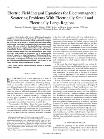
144IEEE TRANSACTIONS ON VISUALIZATION AND COMPUTER GRAPHICS, VOL. 3, NO. 2, APRIL-JUNE 1997disadvantages of these ray casting approaches is that theydo not exploit coherence between nearby rays that maycross the same set of cells.Another approach for rendering irregular grids is theuse of projection (“feed-forward”) methods [22], [45], [34],[38], in which the cells are projected onto the screen, oneby-one, in a visibility ordering, incrementally accumulatingtheir contributions to the final image. One advantage ofthese methods is the ability to use graphics hardware tocompute the volumetric lighting models in order to speedup rendering. Another advantage of this approach is that itworks in object space, allowing coherence to be exploiteddirectly: By projecting cells onto the image plane, we mayend up with large regions of pixels that correspond to rayshaving the same depth ordering, and this is discoveredwithout explicitly casting these rays. However, in order forthe projection to be possible, a depth ordering of the cellshas to be computed, which is, of course, not always possible; even a set of three triangles can have a cyclic overlap.Computing and verifying depth orders is possible in4 3 eOntime [1], [7], [9], where e 0 is an arbitrarily smallejpositive constant. In case no depth ordering exists, it is animportant problem to find a small number of “cuts” thatbreak the objects in such a way that a depth ordering doesexist; see [7], [5]. BSP trees have been used to obtain such adecomposition, but can result in a quadratic number ofpieces [13], [26]. However, for some important classes ofmeshes (e.g., rectilinear meshes and Delaunay meshes [11]),it is known that a depth ordering always exists, with respect to any viewpoint. This structure has been exploitedby Max et al. [22]. Williams [45] has obtained a linear-timealgorithm for visibility ordering convex (connected) acyclicmeshes whose union of (convex) cells is itself convex, assuming a visibility ordering exists. Williams also suggestsheuristics that can be applied in case there is no visibilityordering or in the case of nonconvex meshes, (e.g., by tetrahedralizing the nonconvexities which, unfortunately, mayresult in a quadratic number of cells). In [40], techniques arepresented where no depth ordering is strictly necessaryand, in some cases, calculated approximately. Very fastrendering is achieved by using graphics hardware to project the partially sorted faces.A recent scanline technique that handles multiple andoverlapping grids is presented in [44]. They process the setof polygonal facets of cells, by first bucketing them according to which scanline contains the topmost vertex, and thenmaintaining a “y-actives list” of polygons present at eachscanline, as they sweep from top to bottom (in y). Then, oneach scanline, they scan in x, bucketing polygons accordingto their left extent, and then maintaining (via merging) az-sorted list of polygons, as they scan from left to right. Themethod has been parallelized and used within a multiresolution hierarchy, based on a kD tree.Two other important references on rendering irregulargrids have not yet been discussed here—Giertsen [15] andYagel et al. [47]. We elaborate on these in the next section,as they are closely related to our method.In summary, projection methods are potentially fasterthan ray casting methods, since they exploit spatial coherence. However, projection methods give inaccurate renderings if there is no visibility ordering, and methods tobreak cycles are either heuristic in nature or potentiallycostly in terms of space and time.2 SWEEP-PLANE APPROACHESA standard algorithmic paradigm in computational geometry is the “sweep” paradigm [29]. Commonly, a sweepline is swept across the plane, or a sweep-plane is sweptacross three-space. A data structure, called the sweep structure (or status), is maintained during the simulation of thecontinuous sweep, and at certain discrete events (e.g., whenthe sweep-line hits one of a discrete set of points), thesweep structure is updated to reflect the change. The idea isto localize the problem to be solved, solving it within thelower dimensional space of the sweep-line or sweep-plane.By processing the problem according to the systematicsweeping of the space, sweep algorithms are able to exploitspatial coherence in the data.2.1 Giertsen’s MethodGiertsen’s pioneering work [15] was the first step in optimizingray casting by making use of coherency in order to speed up rendering. He performs a sweep of the mesh in three-space, using asweep-plane that is parallel to the x-z plane. Here, the viewingcoordinate system is such that the viewing plane is the x-y plane,and the viewing direction is the z direction; see Fig. 1. The algorithm consists of the following steps:1) Transform all vertices of S to the viewing coordinatesystem.2) Sort the (transformed) vertices of S by their ycoordinates; put the ordered vertices, as well as they-coordinates of the scanlines for the viewing image,into an event priority queue, implemented in this caseas an array, A.3) Initialize the Active Cell List (ACL) to empty. The ACLrepresents the sweep status; it maintains a list of thecells currently intersected by the sweep-plane.4) While A is not empty, do:a) Pop the event queue: If the event corresponds to avertex, v, then go to b; otherwise, go to c.b) Update ACL: Insert/delete, as appropriate, thecells incident on v. (Giertsen assumed that the cellsare disjoint, so each v belongs to a single cell.)c) Render current scanline: Giertsen uses a memoryhash buffer, based on a regular grid of squares inthe sweep-plane, allowing a straightforward casting of the rays that lie on the current scanline.By sweeping three-space, Giertsen reduces the ray casting problem in three-space to a two-dimensional cell sorting problem.Giertsen’s method has several advantages over previousray casting schemes. First, there is no need to maintain connectivity information between cells of the mesh. (In fact, heassumes the cells are all disjoint.) Second, the computationally expensive ray shooting in three-space is replaced by asimple walk through regular grid cells in a plane. Finally,the method is able to take advantage of coherence from onescanline to the next.However, there are some drawbacks to the method,including:1) The original data is coarsened into a finite resolutionbuffer (the memory hashing buffer) for rendering,

SILVA AND MITCHELL: THE LAZY SWEEP RAY CASTING ALGORITHM FOR RENDERING IRREGULAR GRIDS1453 THE LAZY SWEEP RAY CASTING ALGORITHMThe design of our new method is based on two main goals:1) The depth ordering of the cells should be correctalong the rays corresponding to every pixel; and2) The algorithm should be as efficient as possible, taking advantage of structure and coherence in the data.With the first goal in mind, we chose to develop a newray casting algorithm, in order to be able to handle cyclesamong cells (a case causing difficulties for projection methods). To address the second goal, we use a sweep approach,as did Giertsen, in order to exploit both interscanline andinterray coherence. Our algorithm has the following advantages over Giertsen’s:Fig. 1. A sweep-plane (perpendicular to the y-axis) used in sweepingthree-space.basically limiting the resolution of the rendering, andpossibly creating an aliasing effect. While one couldsimply increase the size of the buffer, this approach isimpractical in large datasets, where the cell sizevariation can be on the order of 1:100,000. Further,Giertsen mentions that when cells get mapped to thesame location, this is considered a degenerate case,and the later cells are ignored; however, this resolution might lead to temporal aliasing when calculatingmultiple images.2) Another disadvantage when comparing to other raycasting techniques is the need to have two copies of thedataset, as the transformation and sorting of the cellsmust be done before the sweeping can be started. (Notethat this is also a feature of cell projection methods.)One cannot just keep retransforming a single copy,since floating point errors could accumulate.2.2 Yagel et al.’s MethodIn [46], [47], Yagel et al. proposed a method that uses asweep-plane parallel to the viewing plane. At each positionof the sweep-plane, the plane is intersected with the grid,resulting in a two-dimensional slice, each of whose cells arethen scan-converted using the graphics hardware in orderto obtain an image of that slice, which can then be composited with the previously accumulated image that resulted from the sweep so far. Several optimizations are possible. For example, instead of performing a full sort alongthe z-direction, a bucketing technique can be used. Also, theintersections of mesh edges with the slices can be accelerated by storing incremental step sizes ('x and 'y) corresponding to the interslice distance ('z); however, this speeduprequires considerably more memory. Furthermore, the storage of the polygons in any given slice requires a significantamount of memory (e.g., 13.4 MB for the Blunt Fin [47]).This method can handle general polyhedral grids without having to compute adjacency information, and, conceptually, it can generate high quality images at the expense of “slice oversampling.” The simplicity of the methodmakes it very attractive for implementation and use.(Ideally, the user should have access to high-performancegraphics hardware and an abundance of memory.)1) It avoids the explicit transformation and sortingphase, thereby avoiding the storage of an extra copyof the vertices;2) It makes no requirements or assumptions about thelevel of connectivity or convexity among cells of themesh; however, it does take advantage of structure inthe mesh, running faster in cases that involve mesheshaving convex cells and convex components;3) It avoids the use of a hash buffer plane, thereby allowing accurate rendering even for meshes whosecells greatly vary in size;4) It is able to handle parallel and perspective projectionwithin the same framework, without explicit transformations.3.1 Performing the SweepOur sweep method, like Giertsen’s, sweeps space with asweep-plane that is orthogonal to the viewing plane (the xy plane), and parallel to the scanlines (i.e., parallel to the x-zplane).Events occur when the sweep-plane hits vertices of themesh S. But, rather than sorting all of the vertices of S inadvance and placing them into an auxiliary data structure(thereby at least doubling the storage requirements), wemaintain an event queue (priority queue) of an appropriate(small) subset of the mesh vertices.A simple (linear-time) preprocessing pass through thedata readily identifies the set of vertices on the boundary ofthe mesh. We initialize the event queue with these boundary vertices, prioritized according to the magnitude of theirinner product (dot product) with the vector representingthe y-axis (“up”) in the viewing coordinate system (i.e., according to their y-coordinates). (We do not explicitly transform coordinates.) Furthermore, at any given instant, theevent queue only stores the set of boundary vertices not yetswept over, plus the vertices that are the upper endpointsof the edges currently intersected by the sweep-plane. Inpractice, the event queue is relatively small, usually accounting for a very small percentage of the total data size.As the sweep takes place, new vertices (nonboundary ones)will be inserted into and deleted from the event queue eachtime the sweep-plane hits a vertex of S.As the sweep algorithm proceeds, we maintain a sweepstatus data structure, which records the necessary information about the current slice through S in an “active

146IEEE TRANSACTIONS ON VISUALIZATION AND COMPUTER GRAPHICS, VOL. 3, NO. 2, APRIL-JUNE 1997edge” list—see Section 5. When the sweep-plane encounters a vertex event (as determined by the event queue),the sweep status and the event queue data structuresmust be updated. In the main loop of the sweep algorithm, we pop the event queue, obtaining the next vertex,v, to be hit, and we check whether or not the sweep-planeencounters v before it reaches the y-coordinate of the nextscanline. If it does hit v first, we perform the appropriateinsertions/deletions on the event queue and the sweepstatus structure; these are easily determined by local tests(checking the signs of dot products) in the neighborhoodof v. Otherwise, the sweep-plane has encountered a scanline. At this point, we stop the sweep and drop into a twodimensional ray casting procedure (also based on asweep) as described below. The algorithm terminates oncethe last scanline is processed.3.2 Processing a ScanlineWhen the sweep-plane encounters a scanline, the current(3D) sweep status data structure gives us a “slice”through the mesh in which we must solve a twodimensional ray casting problem. Let 6 denote the polygonal (planar) subdivision at the current scanline (i.e., 6is the subdivision obtained by intersecting the sweepplane with the mesh S.) In time linear in the size of 6, thesubdivision 6 can be recovered (both its geometry and itstopology) by stepping through the sweep status structureand utilizing the local topology of the cells in the slice.(The sweep status gives us the set of edges intersectingthe sweep plane; these edges define the vertices of 6, andthe edges of 6 can be obtained by searching the set of triangular facets incident on each such edge.) In our implementation, however, 6 is not constructed explicitly, butonly given implicitly by the sweep status data structure (alist of “active edges”), and then locally reconstructed asneeded during the two-dimensional sweep (describedbelow). The details of the implementation are nontrivialand they are presented in Section 5.The two-dimensional ray casting problem is also solvedusing a sweep algorithm—now we sweep the plane with asweep-line parallel to the z axis. (Or, in the case of perspective projection, we sweep with a ray eminating from theviewer’s eye.) Events now correspond to vertices of theplanar subdivision 6, which occur at intersection pointsbetween an “active edge” in the (3D) sweep status and thecurrent sweep-plane. These event points are processed in xorder; thus, we begin by sorting them. (An alternative approach, mentioned in Section 4, is to proceed as we did in3D, by first identifying and sorting only the locally extremalvertices of 6, and then maintaining an event queue duringthe sweep. Since a single slice has relatively few eventpoints compared with the size of S, we opted, in our implementation, simply to sort them outright.) The sweep-linestatus is an ordered list of the segments of 6 crossed by thesweep-line. The sweep-line status is initially empty. Then,as we pass the sweep-line over 6, we update the sweep-linestatus at each event point, making (local) insertions anddeletions as necessary. (This is analogous to the BentleyOttmann sweep that is used for computing line segment intersections in the plane [29].) We also stop the sweep at eachof the x-coordinates that correspond to the rays that we arecasting (i.e., at the pixel coordinates along the current scanline), and output to the rendering model the sorted ordering(depth ordering) given by the current sweep-line status.4 ANALYSIS: UPPER AND LOWER BOUNDSWe now proceed to give a theoretical analysis of the timerequired to render irregular grids. We begin with“negative” results that establish lower bounds on theworst-case running time:THEOREM 1 (Lower Bounds). Let S be a mesh having c connected components and n edges. Even if all cells of S areconvex, W k n log n is a lower bound on the worst-casecomplexity of ray casting. If all cells of S are convex and, foreach connected component of S, the union of cells in the component is convex, then W c log c is a lower bound. Here, k2is the total number of facets crossed by all N rays that arecast through the mesh (one per pixel of the image plane).chchPROOF. It is clear that :(k) is a lower bound, since k is thesize of the output from the ray casting.Let us start with the case of c convex componentsin the mesh S, each made up of a set of convex cells.Assume that one of the rays to be traced lies exactlyalong the z-axis. In fact, we can assume that there isonly one pixel at the origin in the image plane. Then,the only ray to be cast is the one along the z-axis, andk simply measures how many cells it intersects. Toshow a lower bound of W c log c , we simply note thatany ray tracing algorithm that outputs the intersectedcells, in order, along a ray, can be used to sort c numbers, zi. (Just construct, in O(c) time, tiny disjoint tetrahedral cells, one centered on each zi.)Now, consider the case of a connected mesh S, allof whose cells are convex. We assume that all localconnectivity of the cells of S is part of the inputmesh data structure. (The claim of the theorem isthat, even with all of this information, we still musteffectively perform a sort.) Again, we claim thatcasting a single ray along the z-axis will require thatwe effectively sort n numbers, z1, , zn. We take theunsorted numbers zi and construct a mesh S as follows. Take a unit cube centered on the origin andsubtract from it a cylinder, centered on the z-axis,with cross sectional shape a regular 2n-gon, havingradius less than 1/2. Now remove the half of thispolyhedral solid that lies above the x-z plane. Wenow have a polyhedron P of genus 0 that we haveconstructed in time O(n). We refer to the n (skinny)rectangular facets that bound the concavity as the“walls.” Now, for each point (0, 0, zi), create a thin“wedge” that contains (0, 0, zi) (and no other point(0, 0, zj), j i), such that the wedge is attached towall i (and touches no other wall). Refer to Fig. 2.We now have a polyhedron P, still of genus 0, of sizeO(n), and this polyhedron is

142 IEEE TRANSACTIONS ON VISUALIZATION AND COMPUTER GRAPHICS, VOL. 3, NO. 2, APRIL-JUNE 1997 The Lazy Sweep Ray Casting Algorithm for Rendering Irregular Grids Claudio T. Silva and Joseph S.B. Mitchell Abstract— Lazy Sweep Ray Casting is a fast algorithm for renderin