Transcription
tensorflow#tensorflow
Table of ContentsAbout1Chapter 1: Getting started with tensorflow2Remarks2Examples2Installation or Setup2Basic Example2Linear Regression2Tensorflow Basics4Counting to 106Chapter 2: Creating a custom operation with tf.py func (CPU only)7Parameters7Examples7Basic example7Why to use tf.py func7Chapter 3: Creating RNN, LSTM and bidirectional RNN/LSTMs with TensorFlowExamplesCreating a bidirectional LSTMChapter 4: How to debug a memory leak in TensorFlowExamples9991010Use Graph.finalize() to catch nodes being added to the graph10Use the tcmalloc allocator10Chapter 5: How to use TensorFlow Graph Collections?12Remarks12Examples12Create your own collection and use it to collect all your losses.12Collect variables from nested scopes13Chapter 6: Math behind 2D convolution with advanced examples in TF15Introduction15Examples15No padding, strides 115
Some padding, strides 116Padding and strides (the most general case)17Chapter 7: Matrix and Vector ArithmeticExamples1818Elementwise Multiplication18Scalar Times a Tensor18Dot Product19Chapter 8: Measure the execution time of individual operationsExamplesBasic example with TensorFlow's Timeline objectChapter 9: Minimalist example code for distributed uted training exampleChapter 10: Multidimensional softmaxExamples232525Creating a Softmax Output Layer25Computing Costs on a Softmax Output Layer25Chapter 11: Placeholders26Parameters26Examples26Basics of Placeholders26Placeholder with Default27Chapter 12: Q-learningExamplesMinimal ExampleChapter 13: Reading the dataExamples2929293434Count examples in CSV file34Read & Parse TFRecord file34Random shuffling the examples35Reading data for n epochs with batching36
How to load images and labels from a TXT fileChapter 14: Save and Restore a Model in ing the model40Restoring the model41Chapter 15: Save Tensorflow model in Python and load with Java43Introduction43Remarks43Examples43Create and save a model with Python43Load and use the model in Java.43Chapter 16: Simple linear regression structure in TensorFlow with s46Simple regression function code structure46Main Routine47Normalization Routine47Read Data routine47Chapter 17: Tensor indexing49Introduction49Examples49Extract a slice from a tensor49Extract non-contiguous slices from the first dimension of a tensor49Numpy-like indexing using tensors51How to use tf.gather nd52Chapter 18: TensorFlow GPU setup55Introduction55Remarks55
Examples55Run TensorFlow on CPU only - using the CUDA VISIBLE DEVICES environment variable.55Run TensorFlow Graph on CPU only - using tf.config 55Use a particular set of GPU devices56List the available devices available by TensorFlow in the local process.56Control the GPU memory allocation56Chapter 19: Using 1D convolution58Examples58Basic example58Math behind 1D convolution with advanced examples in TF58The easiest way is for padding 0, stride 158Convolution with padding59Convolution with strides60Chapter 20: Using Batch Normalization61Parameters61Remarks61Examples62A Full Working Example of 2-layer Neural Network with Batch Normalization (MNIST Dataset)62Import libraries (language dependency: python 2.7)62load data, prepare data62One-Hot-Encode y63Split training, validation, testing data63Build a simple 2 layer neural network graph63An initialization function63Build Graph64Start a session65Chapter 21: Using if condition inside the TensorFlow graph with tf.cond66Parameters66Remarks66Examples66Basic example66
When f1 and f2 return multiple tensors66define and use functions f1 and f2 with parameters67Chapter 22: Using transposed convolution layers68ExamplesUsing tf.nn.conv2d transpose for arbitary batch sizes and with automatic output shape calcChapter 23: VariablesExamples68687070Declaring and Initializing Variable Tensors70Fetch the value of a TensorFlow variable or a Tensor70Chapter 24: Visualizing the output of a convolutional layer72Introduction72Examples72A basic example of 2 stepsCredits7274
AboutYou can share this PDF with anyone you feel could benefit from it, downloaded the latest versionfrom: tensorflowIt is an unofficial and free tensorflow ebook created for educational purposes. All the content isextracted from Stack Overflow Documentation, which is written by many hardworking individuals atStack Overflow. It is neither affiliated with Stack Overflow nor official tensorflow.The content is released under Creative Commons BY-SA, and the list of contributors to eachchapter are provided in the credits section at the end of this book. Images may be copyright oftheir respective owners unless otherwise specified. All trademarks and registered trademarks arethe property of their respective company owners.Use the content presented in this book at your own risk; it is not guaranteed to be correct noraccurate, please send your feedback and corrections to info@zzzprojects.comhttps://riptutorial.com/1
Chapter 1: Getting started with tensorflowRemarksThis section provides an overview of what tensorflow is, and why a developer might want to use it.It should also mention any large subjects within tensorflow, and link out to the related topics. Sincethe Documentation for tensorflow is new, you may need to create initial versions of those relatedtopics.ExamplesInstallation or SetupAs of Tensorflow version 1.0 installation has become much easier to perform. At minimum toinstall TensorFlow one needs pip installed on their machine with a python version of at least 2.7 or3.3 .pip install --upgrade tensorflowpip3 install --upgrade tensorflow# for Python 2.7# for Python 3.nFor tensorflow on a GPU machine (as of 1.0 requires CUDA 8.0 and cudnn 5.1, AMD GPU notsupported)pip install --upgrade tensorflow-gpu # for Python 2.7 and GPUpip3 install --upgrade tensorflow-gpu # for Python 3.n and GPUTo test if it worked open up the correct version of python 2 or 3 and runimport tensorflowIf that succeeded without error then you have tensorflow installed on your machine.*Be aware this references the master branch one can change this on the link above to referencethe current stable release.)Basic ExampleTensorflow is more than just a deep learning framework. It is a general computation framework toperform general mathematical operations in a parallel and distributed manner. An example of suchis described below.https://riptutorial.com/2
Linear RegressionA basic statistical example that is commonly utilized and is rather simple to compute is fitting a lineto a dataset. The method to do so in tensorflow is described below in code and comments.The main steps of the (TensorFlow) script are:1. Declare placeholders (x ph, y ph) and variables (W, b)2. Define the initialization operator (init)3. Declare operations on the placeholders and variables (y pred, loss, train op)4. Create a session (sess)5. Run the initialization operator (sess.run(init))6. Run some graph operations (e.g. sess.run([train op, loss], feed dict {x ph:x, y ph: y}))The graph construction is done using the Python TensorFlow API (could also be done using theC TensorFlow API). Running the graph will call low-level C routines.'''function: create a linear model which try to fit the liney x 2 using SGD optimizer to minimizeroot-mean-square(RMS) loss function'''import tensorflow as tfimport numpy as np# number of epochnum epoch 100# training data x and label yx np.array([0., 1., 2., 3.], dtype np.float32)y np.array([2., 3., 4., 5.], dtype np.float32)# convert x and y to 4x1 matrixx np.reshape(x, [4, 1])y np.reshape(y, [4, 1])# test set(using a little trick)x test x 0.5y test y 0.5# This part of the script builds the TensorFlow graph using the Python API# First declare placeholders for input x and label y# Placeholders are TensorFlow variables requiring to be explicitly fed by some# input datax ph tf.placeholder(tf.float32, shape [None, 1])y ph tf.placeholder(tf.float32, shape [None, 1])###W#bVariables (if not specified) will be learnt as the GradientDescentOptimizeris runDeclare weight variable initialized using a truncated normal law tf.Variable(tf.truncated normal([1, 1], stddev 0.1))Declare bias variable initialized to a constant 0.1 tf.Variable(tf.constant(0.1, shape [1]))https://riptutorial.com/3
# Initialize variables just declaredinit tf.initialize all variables()# In this part of the script, we build operators storing operations# on the previous variables and placeholders.# model: y w * x by pred x ph * W b# loss functionloss tf.mul(tf.reduce mean(tf.square(tf.sub(y pred, y ph))), 1. / 2)# create training graphtrain op ss)# This part of the script runs the TensorFlow graph (variables and operations# operators) just built.with tf.Session() as sess:# initialize all the variables by running the initializer operatorsess.run(init)for epoch in xrange(num epoch):# Run sequentially the train op and loss operators with# x ph and y ph placeholders fed by variables x and y, loss val sess.run([train op, loss], feed dict {x ph: x, y ph: y})print('epoch %d: loss is %.4f' % (epoch, loss val))# see what model do in the test set# by evaluating the y pred operator using the x test datatest val sess.run(y pred, feed dict {x ph: x test})print('ground truth y is: %s' % y test.flatten())print('predict y is: %s' % test val.flatten())Tensorflow BasicsTensorflow works on principle of dataflow graphs. To perform some computation there are twosteps:1. Represent the computation as a graph.2. Execute the graph.Representation: Like any directed graph a Tensorflow graph consists of nodes and directionaledges.Node: A Node is also called an Op(stands for operation). An node can have multiple incomingedges but single outgoing edge.Edge: Indicate incoming or outgoing data from a Node. In this case input(s) and output of someNode(Op).Whenever we say data we mean an n-dimensional vector known as Tensor. A Tensor has threeproperties: Rank, Shape and Type Rank means number of dimensions of the Tensor(a cube or box has rank 3). Shape means values of those dimensions(box can have shape 1x1x1 or 2x5x7). Type means datatype in each coordinate of Tensor.https://riptutorial.com/4
Execution: Even though a graph is constructed it is still an abstract entity. No computationactually occurs until we run it. To run a graph, we need to allocate CPU resource to Ops inside thegraph. This is done using Tensorflow Sessions. Steps are:1. Create a new session.2. Run any Op inside the Graph. Usually we run the final Op where we expect the output of ourcomputation.An incoming edge on an Op is like a dependency for data on another Op. Thus when we run anyOp, all incoming edges on it are traced and the ops on other side are also run.Note: Special nodes called playing role of data source or sink are also possible. For example youcan have an Op which gives a constant value thus no incoming edges(refer value 'matrix1' in theexample below) and similarly Op with no outgoing edges where results are collected(refer value'product' in the example below).Example:import tensorflow as tf# Create a Constant op that produces a 1x2 matrix. The op is# added as a node to the default graph.## The value returned by the constructor represents the output# of the Constant op.matrix1 tf.constant([[3., 3.]])# Create another Constant that produces a 2x1 matrix.matrix2 tf.constant([[2.],[2.]])# Create a Matmul op that takes 'matrix1' and 'matrix2' as inputs.# The returned value, 'product', represents the result of the matrix# multiplication.product tf.matmul(matrix1, matrix2)# Launch the default graph.sess tf.Session()# To run the matmul op we call the session 'run()' method, passing 'product'# which represents the output of the matmul op. This indicates to the call# that we want to get the output of the matmul op back.https://riptutorial.com/5
## All inputs needed by the op are run automatically by the session. They# typically are run in parallel.## The call 'run(product)' thus causes the execution of three ops in the# graph: the two constants and matmul.## The output of the op is returned in 'result' as a numpy ndarray object.result sess.run(product)print(result)# [[ 12.]]# Close the Session when we're done.sess.close()Counting to 10In this example we use Tensorflow to count to 10. Yes this is total overkill, but it is a nice exampleto show an absolute minimal setup needed to use Tensorflowimport tensorflow as tf# create a variable, refer to it as 'state' and set it to 0state tf.Variable(0)# set one to a constant set to 1one tf.constant(1)# update phase adds state and one and then assigns to stateaddition tf.add(state, one)update tf.assign(state, addition )# create a sessionwith tf.Session() as sess:# initialize session variablessess.run( tf.global variables initializer() )print "The starting state is",sess.run(state)print "Run the update 10 times."for count in range(10):# execute the updatesess.run(update)print "The end state is",sess.run(state)The important thing to realize here is that state, one, addition, and update don't actually containvalues. Instead they are references to Tensorflow objects. The final result is not state, but insteadis retrieved by using a Tensorflow to evaluate it using sess.run(state)This example is from https://github.com/panchishin/learn-to-tensorflow . There are several otherexamples there and a nice graduated learning plan to get acquainted with manipulating theTensorflow graph in python.Read Getting started with tensorflow online: ngstarted-with-tensorflowhttps://riptutorial.com/6
Chapter 2: Creating a custom operation withtf.py func (CPU only)ParametersParameterDetailsfuncpython function, which takes numpy arrays as its inputs and returns numpyarrays as its outputsinplist of Tensors (inputs)Toutlist of tensorflow data types for the outputs of funcExamplesBasic exampleThe tf.py func(func, inp, Tout) operator creates a TensorFlow operation that calls a Pythonfunction, func on a list of tensors inp.See the documentation for tf.py func(func,inp, Tout).Warning: The tf.py func() operation will only run on CPU. If you are using distributedTensorFlow, the tf.py func() operation must be placed on a CPU device in the same process asthe client.def func(x):return 2*xx tf.constant(1.)res tf.py func(func, [x], [tf.float32])# res is a list of length 1Why to use tf.py funcThe tf.py func() operator enables you to run arbitrary Python code in the middle of a TensorFlowgraph. It is particularly convenient for wrapping custom NumPy operators for which no equivalentTensorFlow operator (yet) exists. Adding tf.py func() is an alternative to using sess.run() callsinside the graph.Another way of doing that is to cut the graph in two parts:# Part 1 of the graphinputs . # in the TF graphhttps://riptutorial.com/7
# Get the numpy array and apply funcval sess.run(inputs) # get the value of inputsoutput val func(val) # numpy array# Part 2 of the graphoutput tf.placeholder(tf.float32, shape .)train op .# We feed the output val to the tensor outputsess.run(train op, feed dict {output: output val})With tf.py func this is much easier:# Part 1 of the graphinputs .# call to tf.py funcoutput tf.py func(func, [inputs], [tf.float32])[0]# Part 2 of the graphtrain op .# Only one call to sess.run, no need of a intermediate placeholdersess.run(train op)Read Creating a custom operation with tf.py func (CPU only) u-only-https://riptutorial.com/8
Chapter 3: Creating RNN, LSTM andbidirectional RNN/LSTMs with TensorFlowExamplesCreating a bidirectional LSTMimport tensorflow as tfdims, layers 32, 2# Creating the forward and backwards cellslstm fw cell tf.nn.rnn cell.BasicLSTMCell(dims, forget bias 1.0)lstm bw cell tf.nn.rnn cell.BasicLSTMCell(dims, forget bias 1.0)# Pass lstm fw cell / lstm bw cell directly to tf.nn.bidrectional rnn# if only a single layer is neededlstm fw multicell tf.nn.rnn cell.MultiRNNCell([lstm fw cell]*layers)lstm bw multicell tf.nn.rnn cell.MultiRNNCell([lstm bw cell]*layers)# tf.nn.bidirectional rnn takes a list of tensors with shape# [batch size x cell fw.state size], so separate the input into discrete# timesteps.X tf.unpack(state below, axis 1)# state fw and state bw are the final states of the forwards/backwards LSTM, respectivelyoutputs, state fw, state bw tf.nn.bidirectional rnn(lstm fw multicell, lstm bw multicell,X, dtype 'float32')Parameters is a 3D tensor of with the following dimensions: [batch size, maximum sequenceindex, dims]. This comes from a previous operation, such as looking up a word embedding. dims is the number of hidden units. layers can be adjusted above 1 to create a stacked LSTM network.state belowNotes may not be able to determine the size of a given axis (use the nums argument if thisis the case). It may be helpful to add an additional weight bias multiplication beneath the LSTM (e.g.tf.matmul(state below, U) b.tf.unpackRead Creating RNN, LSTM and bidirectional RNN/LSTMs with TensorFlow withtensorflowhttps://riptutorial.com/9
Chapter 4: How to debug a memory leak inTensorFlowExamplesUse Graph.finalize() to catch nodes being added to the graphThe most common mode of using TensorFlow involves first building a dataflow graph ofTensorFlow operators (like tf.constant() and tf.matmul(), then running steps by calling thetf.Session.run() method in a loop (e.g. a training loop).A common source of memory leaks is where the training loop contains calls that add nodes to thegraph, and these run in every iteration, causing the graph to grow. These may be obvious (e.g. acall to a TensorFlow operator like tf.square()), implicit (e.g. a call to a TensorFlow library functionthat creates operators like tf.train.Saver()), or subtle (e.g. a call to an overloaded operator on atf.Tensor and a NumPy array, which implicitly calls tf.convert to tensor() and adds a newtf.constant() to the graph).The tf.Graph.finalize() method can help to catch leaks like this: it marks a graph as read-only,and raises an exception if anything is added to the graph. For example:loss .train op oss)init tf.initialize all variables()with tf.Session() as sess:sess.run(init)sess.graph.finalize() # Graph is read-only after this statement.for in range(1000000):sess.run(train op)loss sq tf.square(loss)sess.run(loss sq)# Exception will be thrown here.In this case, the overloaded * operator attempts to add new nodes to the graph:loss .# .with tf.Session() as sess:# .sess.graph.finalize() # Graph is read-only after this statement.# .dbl loss loss * 2.0 # Exception will be thrown here.Use the tcmalloc allocatorTo improve memory allocation performance, many TensorFlow users often use tcmalloc instead ofthe default malloc() implementation, as tcmalloc suffers less from fragmentation when allocatinghttps://riptutorial.com/10
and deallocating large objects (such as many tensors). Some memory-intensive TensorFlowprograms have been known to leak heap address space (while freeing all of the individual objectsthey use) with the default malloc(), but performed just fine after switching to tcmalloc. In addition,tcmalloc includes a heap profiler, which makes it possible to track down where any remainingleaks might have occurred.The installation for tcmalloc will depend on your operating system, but the following works onUbuntu 14.04 (trusty) (where script.py is the name of your TensorFlow Python program): sudo apt-get install google-perftools4 LD PRELOAD /usr/lib/libtcmalloc.so.4 python script.py .As noted above, simply switching to tcmalloc can fix a lot of apparent leaks. However, if thememory usage is still growing, you can use the heap profiler as follows: LD PRELOAD /usr/lib/libtcmalloc.so.4 HEAPPROFILE /tmp/profile python script.py .After you run the above command, the program will periodically write profiles to the filesystem.The sequence of profiles will be named: /tmp/profile.0000.heap /tmp/profile.0001.heap /tmp/profile.0002.heap .You can read the profiles using the google-pprof tool, which (for example, on Ubuntu 14.04) can beinstalled as part of the google-perftools package. For example, to look at the third snapshotcollected above: google-pprof --gv which python /tmp/profile.0002.heapRunning the above command will pop up a GraphViz window, showing the profile information as adirected graph.Read How to debug a memory leak in TensorFlow /riptutorial.com/11
Chapter 5: How to use TensorFlow GraphCollections?RemarksWhen you have huge model, it is useful to form some groups of tensors in your computationalgraph, that are connected with each other. For example tf.GraphKeys class contains such standartcollections as:tf.GraphKeys.VARIABLEStf.GraphKeys.TRAINABLE VARIABLEStf.GraphKeys.SUMMARIESExamplesCreate your own collection and use it to collect all your losses.Here we will create collection for losses of Neural Network's computational graph.First create a computational graph like so:with tf.variable scope("Layer"):W tf.get variable("weights", [m, k],initializer tf.zeros initializer([m, k], dtype tf.float32))b1 tf.get variable("bias", [k],initializer tf.zeros initializer([k], dtype tf.float32))z tf.sigmoid((tf.matmul(input, W) b1))with tf.variable scope("Softmax"):U tf.get variable("weights", [k, r],initializer tf.zeros initializer([k,r], dtype tf.float32))b2 tf.get variable("bias", [r],initializer tf.zeros initializer([r], dtype tf.float32))out tf.matmul(z, U) b2cross entropy tf.reduce mean(tf.nn.sparse softmax cross entropy with logits(out, labels))To create a new collection, you can simply start calling tf.add to collection() - the first call willcreate the collection.tf.add to collection("my losses",self.config.l2 * (tf.add n([tf.reduce sum(U ** 2), tf.reduce sum(W ** 2)])))tf.add to collection("my losses", cross entropy)And finally you can get tensors from your collection:loss sum(tf.get collection("my losses"))https://riptutorial.com/12
Note that tf.get collection() returns a copy of the collection or an empty list if the collection doesnot exist. Also, it does NOT create the collection if it does not exist. To do so, you could usetf.get collection ref() which returns a reference to the collection and actually creates an emptyone if it does not exist yet.Collect variables from nested scopesBelow is a single hidden layer Multilayer Perceptron (MLP) using nested scoping of variables.def weight variable(shape):return tf.get variable(name "weights", shape shape,initializer tf.zeros initializer(dtype tf.float32))def bias variable(shape):return tf.get variable(name "biases", shape shape,initializer tf.zeros initializer(dtype tf.float32))def fc layer(input, in dim, out dim, layer name):with tf.variable scope(layer name):W weight variable([in dim, out dim])b bias variable([out dim])linear tf.matmul(input, W) boutput tf.sigmoid(linear)with tf.variable scope("MLP"):x tf.placeholder(dtype tf.float32, shape [None, 1], name "x")y tf.placeholder(dtype tf.float32, shape [None, 1], name "y")fc1 fc layer(x, 1, 8, "fc1")fc2 fc layer(fc1, 8, 1, "fc2")mse loss tf.reduce mean(tf.reduce sum(tf.square(fc2 - y), axis 1))The MLP uses the the top level scope name MLP and it has two layers with their respective scopenames fc1 and fc2. Each layer also has its own weights and biases variables.The variables can be collected like so:trainable var key tf.GraphKeys.TRAINABLE VARIABLESall vars tf.get collection(key trainable var key, scope "MLP")fc1 vars tf.get collection(key trainable var key, scope "MLP/fc1")fc2 vars tf.get collection(key trainable var key, scope "MLP/fc2")fc1 weight vars tf.get collection(key trainable var key, scope "MLP/fc1/weights")fc1 bias vars tf.get collection(key trainable var key, scope "MLP/fc1/biases")The values of the variables can be collected using the sess.run() command. For example if wewould like to collect the values of the fc1 weight vars after training, we could do the following:sess tf.Session()# add code to initialize variables# add code to train the network# add code to create test data x test and y testfc1 weight vals sess.run(fc1, feed dict {x: x test, y: y test})print(fc1 weight vals) # This should be an ndarray with ndim 2 and shape [1, 8]https://riptutorial.com/13
Read How to use TensorFlow Graph Collections? /riptutorial.com/14
Chapter 6: Math behind 2D convolution withadvanced examples in TFIntroduction2D convolution is computed in a similar way one would calculate 1D convolution: you slide yourkernel over the input, calculate the element-wise multiplications and sum them up. But instead ofyour kernel/input being an array, here they are matrices.ExamplesNo padding, strides 1This is the most basic example, with the easiest calculations. Let's assume your input and kernelare:When you your kernel you will receive the following output:following way: , which is calculated in the14 4 * 1 3 * 0 1 * 1 2 * 2 1 * 1 0 * 0 1 * 0 2 * 0 4 * 16 3*1 1*0 0*1 1*2 0*1 1*0 2*0 4*0 1*16 2*1 1*0 0*1 1*2 2*1 4*0 3*0 1*0 0*112 1 * 1 0 * 0 1 * 1 2 * 2 4 * 1 1 * 0 1 * 0 0 * 0 2 * 1TF's conv2d function calculates convolutions in batches and uses a slightly different format. For aninput it is [batch, in height, in width, in channels] for the kernel it is [filter height,filter width, in channels, out channels]. So we need to provide the data in the correct format:import tensorflow as tfk tf.constant([[1, 0, 1],[2, 1, 0],[0, 0, 1]], dtype tf.float32, name 'k')i tf.constant([[4, 3, 1, 0],[2, 1, 0, 1],[1, 2, 4, 1],[3, 1, 0, 2]], dtype tf.float32, name 'i')kernel tf.reshape(k, [3, 3, 1, 1], name 'kernel')https://riptutorial.com/15
image tf.reshape(i, [1, 4, 4, 1], name 'image')Afterwards the convolution is computed with:res tf.squeeze(tf.nn.conv2d(image, kernel, [1, 1, 1, 1], "VALID"))# VALID means no paddingwith tf.Session() as sess:print sess.run(res)And will be equivalent to the one we calculated by hand.Some padding, strides 1Padding is just a fancy name of telling: surround your input matrix with some constant. In most ofthe cases the constant is zero and this is why people call it zero padding. So if you want to use apadding of 1 in our original input (check the first example with padding 0, strides 1), the matrix willlook like this:To calculate the values of the convolution you do the same sliding. Notice that in our case manyvalues in the middle do not need to be recalculated (they will be the same as in previous example.I also will not show all the calculations here, because the idea is straight-forward. The result is:where 5 0*1 0*0 0*1 0*2 4*1 3*0 0*0 0*1 1*1 . 6 4*1 1*0 0*1 0*2 2*1 0*0 0*0 0*0 0*1TF does not support an arbitrary padding in conv2d function, so if you need some padding that isnot supported, use tf.pad(). Luckily for our input the padding 'SAME' will be equal to padding 1.So we need to change almost nothing in our previous example:res tf.squeeze(tf.nn.conv2d(image, kernel, [1, 1, 1, 1], "SAME"))# 'SAME' makes sure that our output has the same size as input and# uses appropriate padding. In our case it is 1.with tf.Session() as sess:https://riptutorial.com/16
print sess.run(res)You can verify that the answer will be the same as calculated by hand.Padding and strides (the most general case)Now we will apply a strided convolution to our previously described padded example and calculatethe convolution where p 1, s 2Previously when we used strides 1, our slided window moved by 1 position, with strides s itmoves by s positions (you need to calculate s 2 elements less. But in our case we can take ashortcut and do not perform any computations at all. Because we already computed the values fors 1, in our case we can just grab each second element.So if the solution is case of sin case of s 2 1wasit will be:Check the positions of values 14, 2, 12, 6 in the previous matrix. The only change we need toperform in our code is to change the strides from 1 to 2 for width and height dimension (2-nd, 3rd).res tf.squeeze(tf.nn.conv2d(image, kernel, [1, 2, 2, 1], "SAME"))with tf.Session() as sess:print sess.run(res)By the way, there is nothing that stops us from using different strides for different dimensions.Read Math behind 2D convolution with advanced examples in TF es-in-tfhttps://riptutorial.com/17
Chapter 7: Matrix and Vector ArithmeticExamplesElementwise MultiplicationTo perform elementwise multiplication on tensors, you can use either of the following: a*btf.multiply(a, b)Here is a full example of elementwise multiplication using both methods.import tensorflow as tfimport numpy as np# Build a graphgraph tf.Graph()with graph.as default():# A 2x3 matrixa tf.constant(np.array([[ 1, 2, 3],[10,20,30]]),dtype tf.float32)# Another 2x3 matrixb tf.constant(np.array([[2, 2, 2],[3, 3, 3]]),dtype tf.float32)# Elementwise multiplicationc a * bd tf.multiply(a, b)# Run a Sessionwith tf.Session(graph graph) as session:(output c, output d) session.run([c, d])print("output c")print(output c)print("\noutput d")print(output d)Prints out the following:output c[[ 2.4.[ 30. 60.6.]90.]]output d[[ 2.4.[ 30. 60.6.]90.]]Scalar Times a Ten
extracted from Stack Overflow Documentation, which is written by many hardworking individuals at Stack Overflow. It is neither affiliated with Stack Overflow nor official tensorflow. The content is released under Creative Commons BY-SA, and the list of contributors to each chapter are