Transcription
Introduction to TensorFlowFilippo Aleotti, Università di BolognaCorso di Sistemi Digitali MStefano Mattoccia, Università di Bologna
What is TensorFlowTensorflow is an open source machine learning and deeplearning framework developed by Google.It allows to develop machine learning models, and it hasa great support also for deploying.Nowadays widely used in productions not only by Google but also by manyother companies
What is TensorFlowTensorFlow offers API for Python, Java and C/C In this course we will use TensorFlow 1.x, even if the new version ofTensorFlow called TensorFlow 2 is going to be released (but it has a differentparadigm with respect to the previous version)In TensorFlow 1.x, there exist two phases : the building of the graph and theexecution of it.Models trained with TensorFlow may be ported on mobile devices (iOS andAndroid) using a lightweight version of TensorFlow called tf-lite
What is a TensorInformally, a tensor is a multi-dimensional array A 0-D tensor is a scalarA 1-D tensor is an arrayA 2-D tensor is a matrixA 3-D tensor is an array of matrices.
What is a TensorWe can think an image as a 3-D tensor with height H, width W and channeldimensions CPicture from Wikipedia
GraphAs we said before, TensorFlow keeps divided the execution phase from thegraph construction.The graph specifies what operations perform, and how the tensors have to flowfrom the inputs in order to generate the desired outputInternally, the compiler can exploit pruning operations to cut off unusedbranches of the graph, saving memory and computational time
GraphSuppose we have two scalar tensors, x and y, and we need to compute the dotproduct between themThe resulting graph is
GraphOf course, we can build more complex graphs
GraphIn the graph, we have edges and nodes: edges: they represent tensors that flow between nodes nodes: they are tf.Operation added to the graph. They take zero or moreinput tensors and generate zero or more output tensors.In the dot example, x,y and dot are Tensors, while mul is an Operation
TensorIn the previous example we used the tf.Variable to represent both x and yIn TensorFlow we can represent data using various types of tensors: Variable: tensor whose value may change by running operations on it Constant: it creates a constant tensor Placeholders: used to feed the graph with input values during theexecution
Tensor: rank and shapeThe rank of a Tensor is the number of dimensions, while its shape is thenumber of elements in each dimensionRankEntityShapeExample0Scalar[]A single number1Array[N0]A list of numbers2Matrix[N0,N1]A matrix33-Tensor[N0, N1, N2]An image44-Tensor[N0, N1, N2, N3]A batch of images
TensorWhat is the rank of x? And of y?To answer these questions, just print the two ranks and look at the results!
TensorEven if it sounds strange at a first look, the previous result makes sense:In fact, we have asked to TensorFlow the rank of the two Tensors, and it addedto the graph the operation to get itWhat we printed out was the shape of the resulting ranking Tensor (generatedby the rank operation) and not the rank value!To get the rank, we have to execute the graph: at the end of the execution, theranking tensor will assume the rank value
ExecutionIn TensorFlow, the execution of the graph have to be performed inside aSession.The Session takes a graph and it executes all the Operations from the startingpoint up to the desired set of Tensor we want to evaluate.If no graph is selected, the default graph would be used.
Execution: SessioninputsOutsideTensorFlowGraph DefinitionGraph executioninside a SessionInside TensorFlowoutputsOutsideTensorFlow
Execution: SessionWe can create a new Session using the with statement, in order to open andclose automatically the Session (releasing resources at the end):
Execution: SessionIn the previous snapshot we: Created a new Session, called session, with a configuration Config. In theconfig we asked the soft placement option: if no GPU is available (or if anOperation doesn’t have a GPU implementation), than the CPU is the targetdevice We initialized all local and global variables. This step is used to allocateand place onto the right device the previously defined (and added to thegraph) variable. We run both local and global initialization ops since wemay have placed some variables in the LOCAL set of variables (by defaultvariables are GLOBAL)
Execution: Session We asked the Session to run the Graph to get us back the value assumedby the dot Tensor Finally, we printed dot value, dot and their types. As we notice before, dotis a Tensor object (so, related to TensorFlow), but dot value is a scalar (aswe expected) with type np.float32
Execution: SessionLet’s try again with the rank exampleRunning the two rank operations (notice that we used a single session.run with alist as input), now TensorFlow is getting us the expected ranks.
ExecutionTo summarize: TensorFlow has got two phases: the graph creation and its executionSome operations are performed during the first phase, while othersduring the second one.An example of this is a piece of code inside an if statement: since the if isevaluated during the graph construction, that block will add or not a branch inthe graph, but at runtime the new branch will be always executed (if it hasbeen added) or never (if the condition was not satisfied during the graphcreation).If you need to check a condition at runtime, you have to use the tf.cond op.
About TensorFlow versionsTensorFlow has been released in many version (last release in November2019 is r1.15).Some releases may expose different functions and modules from the others,but since there exists a lot of previous code all the versions remain available.The scripts presented in these slides can be run even with newest (e.g., tf1.15) TensorFlow releases, but some warning will be displayed: for instance,in newer versions tf.Session is deprecated in favour of tf.compact.v1.Session.
ShapesAnother example of this dualism concerns the shape: to get the shape of aTensor we can run the following operationsWhy two operations? Are them the same? Let’s look what they print outSo, they are not the same since the first returns a Tensor while the other a list
ShapesHowever, running the Tensor we are getting the right shapeWhat is happening here is that we are asking for two different shapes: thestatic and the dynamicThe former is the shape used at graph creation, while the latter is the shapeassumed by the tensors when we run the graph in the session.
ShapesIn the previous case, the two shapes were equal, but sometimes it happensthat they are not.In particular, the dynamic shape (i.e., the one we get with tf.shape) will alwaysassume a value, since at runtime a specific Tensor with a given shape will flowthrough the graph, while the static shape may not.The static shape represents the shape of a Tensor while we are building thegraph, and we may do not know its shape (or we might know just a portion ofit)!For instance, when we test a trained CNN on images, we might expect imageswith 3 channels (RBG), but we do not impose any constraint about height andwidth
Loading dataIn the previous example we initialized two variables to perform their product.However, a common approach (e.g., when training a neural network) consistsin reading the data from a dataset, typically stored in the file system of yourmachineHow can we load data in our sessions with less binding constraints?
Loading data: placeholdersTensorFlow offers many solutions to load the data you need.Placeholders are a simple yet effective way to load data. As the namesuggests, they stand for somethings else that we currently do not know: atcreation time, we can exploit the placeholder to perform operations, then in thesession.run we will run the graph assigning to each placeholder a specific valueUsing the feed dict method when calling the session.run, we force theplaceholder to assume the given valueUsing placeholders, the graph remains the same, since we are just feeding thesame graph with different values
Loading data: placeholdersIn this case, we are feeding the graph first with the 2x2 matrix [[1,5], [3,2]],then with the 1x2 matrix [3,2].
Loading data: placeholders and static shapeMoreover, you can also notice that we do not specified the full static shape ofthe placeholder: since we created a placeholder with shape [None, 2], atruntime the program expects N couples (with N 1).Exploiting this feature of the static shape we can run firstly giving a 2x2 matrixand then with a 1x2 matrix, but we could have used any Nx2 matrix as input!Let’s look the static shape:
Loading data: placeholders and static shapeNote that the shape of tensor is (2,) since we know that the placeholder hasrank 2 (so we expect two dimensions)On the other hand, the dynamic shape looks like:Notice that we are able to obtain more than a single value using the same runjust passing a list!
Loading data: tf.DataEven if Placeholders are useful to feed the network with arbitrary values,TensorFlow offers complex and more powerful instruments to handle inputdata: tf.Datatf.Data allows us to build a pipeline that may include the loading of your data,their handling (e.g., data augmentation to enlarge the dataset) and how to feedthese data to your network (e.g., data shuffling and batch creation)
Neural NetworkConcepts
Neural Network ConceptsA Neural Network (and also a Convolutional Neural Network) can be seen as aset of weights that, linked together to form a particular architecture, is able toturn the input into the desired (hopefully) outputEach weight is represented in general using a float32 variable, but to preservespace and increase speed sometimes also int32, int16 or even int8 are used.In general, at the beginning these weights are initialized randomly (usually,values are random but there exists some rules to follow, e.g. He initialization),and during the training the weights are updated to obtain better and betterresults.
Neural Network Concepts: loss functionsIn order to understand if we are moving in the right direction (i.e., our outputsare not noise but correct ones) we need a loss (cost) function: the lossmeasures the error we are making giving back as result that output.For many tasks the loss function may be a distance function (e.g., l1 distance,l2 distance and so on), but actually it depends on the final goal.If we measure the distance between our predictions and the desired, perfectoutcomes then our training is supervised. On the contrary, if we minimise theprediction without any kind of label, than the training is called unsupervised.
Neural Network Concepts: monocular depth estimation exampleFor instance, suppose you have to estimate the depth starting from a singleimage (monocular depth estimation).Supervised training: you have to collect a dataset in which each training imageis coupled with its relative ground truth (i.e., a depth value for each pixel).Obtaining ground truth values may be hard and expensive, since you have touse active sensors to obtain better results. The loss function is the distancebetween ground truth and predictions. ExpensiveUnsupervised training: your dataset is made up by standard rgb images, noactive sensors are needed (except if you want to realise also a testing split).You might train your network using image reconstruction techniques based onstereo sequences or monocular sequences. Your loss function may be aphotometric similarity between images. Cheap
Neural Network Concepts: gradientHowever, how can we obtain better weights (so lower costs)?We could move randomly in the variable space but of course it is not feasible!In fact, the number of variables may be extremely large (millions of variables),so we would obtain the minimum of a set of hypothesis if we sample randomlyfrom this space.A better method consists in following the gradient of the function: the gradientis the vector that contains all the partial derivatives of the function at a givenpoint.The gradient points to the direction of greatest increase of the function
Neural Network Concepts: minimisationSo, given a differentiable loss L, function of the weights of the network, we areable to minimise it iteratively estimating the gradient of the loss and “moving”in the opposite direction.In other terms, given the current state of the weights, we have to measure theerror that our network is committing (this error is function of the weights), thenupdate each weight in the opposite direction of the gradient.α is the learning rate, the hyperparameter that rules the “intensity” of thechange.
Neural Network Concepts: backpropagationWe can obtain automatically the partial derivatives that compose the gradientexploiting the chain rule of derivatives: given two functions of x, f and g, thanthe derivative of f ( g (x) ) is f ’ ( g (x) ) * g ’(x).In other terms:We can use this property to obtain the partial derivative of each weight withrespect to the loss function.
Neural Network Concepts: referencesDetailed information about CNN and backpropagation can be found in theConvolutional Neural Network for Visual Recognition course realised byStanford University.Slides can be found hereTensorFlow is able to calculate derivatives automatically exploiting chain rule!
Example
Handwritten digit recognitionIn this example, we are going to build our first Neural Network (in particular, aConvolutional Neural Network) with TensorFlowThe network has to recognise handwritten digit, so given a picture of a numberbetween 0 and 9 the task of the network is to give back to us a scalarrepresentative of that numberCNN2
Example: handwritten digit recognitionIn this example we will use the MNIST Dataset, a collection of 70 000handwritten digit with ground-truth labels. The dataset is made up by 60 000training images and 10 000 testing images.Instead, the network we are going to build is similar to the LeNet-5 network, aCNN proposed by Yann LeCun and Yoshua Bengio.LeNet is a simple yet effective handwritten recognizer proposed (in its firstversion) in 1998. Nowadays, there exists complex and more accurate networks,but it is a good starting point to get acquainted with CNNs
Example: datasetFirst of all, we have to download the MNIST dataset from hereThe dataset is composed by 60 000 28x28 handwritten digit images. Eachimage has a ground-truth labelWe are going to use a split of 53600 images for training the network, and theremaining 6400 for validation. Once the network has been trained, we test it onthe test split, made up of other 10 000 images.Do you know why validation is important? What are the differences withtesting?NOTE: the dataset doesn’t contain a validation split. We are going to extract itdirectly from the training one.
Example: datasetOnce the full dataset (training test) has been downloaded, put those files intothe same folder called, for instance, MNISTyour path/MNIST/- train-images-idx3-ubyte - train-labels-idx1-ubyte- t10k-labels-idx1-ubyte- t10k-images-idx3-ubyteThen, just run the mnist converter.py script to extract the datasetThe script will create three folders: train, test and validation. Each folder willcontain an images folder and a labels.txt file
Example: dataloaderImages have been stored as grayscale pngLet’s prepare the portion of the script in charge of loading our data: the DataLoader.Some considerations: For training, we can use 2 placeholders: one for loading the images andone for their relative labels. We also know that images are 28x28x1Feeding the network just a single example at each step may lead to noiseduring the backprop. A better solution consists in feeding the network witha larger training batch (e.g., 10 or 100)During the training, it is preferable to shuffle the samples, avoiding anyform of relationship due to the data loading
Example: dataloaderIn the following script, we load a training batch selecting the elements in arandom way. You may notice also that we normalize the images (dividing by255)
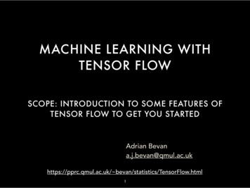
Example: networkC1S2C3S4C5F6OThe network is composed by 5 layers of 3 different types: Convolutional layers (C1, C3) with 5x5 kernels and stride 1Max pooling layers (S2, S4) with 2x2 kernels and stride 2Fully Connected (FC) layers (C5, F6, O) with 120, 84, 10 neurons2
Example: convolutional blockTo create a convolutional block, we can use the following functionIn the function, we first create the weights and the biases for the kernel andthen we apply the convolution between the inputs and the kernel, adding thebiases as the last step.
Example: networkNow, we have got all the building blocks for setting up our network
Example: networkIn the previous snapshot, we used the conv2d block to build the C1 and C3layers, the native tf.nn.max pool for the pooling layers S2 and S4 and thetf.contrib.layers.fully connected for the FC layersWe used the tf.tanh activation functionto add non linearity.The tanh is bounded between -1 and 1and it is differentiable.
Example: loss functionOnce the network has been defined, we need a loss function. Remember thatwe are considering a classification scenario.Each training image has a corresponding label (we stored these labels in thelabels.txt file): our loss function have to receive as input the labels and thepredictions of the network and return a measure of the distance between them.Moreover, the network predicts 10 values (one for each digit) while the correctlabel is just one. We have to transform each label in a so called One-Hot vector,a vector with a single 1 (in correspondence of the ground-truth value) and 0 forall the remainings.7 - [0,0,0,0,0,0,0,1,0,0]
Example: loss functionA common and largely used loss function for object classification is theCross-Entropy loss, which measure the distance between two distributions.In the build loss function we applied the cross entropy between the two vector,then we reduce all the cross-entropy result (one for each sample in the trainingbatch) to a single scalar value applying the mean reduction
Example: cross entropyIn the information theory field, it measures the error we commit using thedistribution q instead of the true distribution pSupposing that p and q are probability distributions, the cross entropymeasures the distance between them. Our desire is to make the modeldistribution as closer as possible to the empirical distribution (the real one).How we can turn p and q into probability distributions? Using the softmax!
Example: softmaxThe softmax σ is defined as normalized exponential function:Doing so, we are dividing the exponential of each network prediction z by thesum of the exponentials. The exponential makes even larger large predictions,and the normalization ensures that: each result will be in the range [0,1]they will sum up to 1they are all 0 .
Example: softmaxIn other words, each result can be seen as a probability!What we desire is a high probability for the correct class and near zeroprobability for others.NOTE: for numerical stability, in TensorFlow the softmax is performed insidethe cross-entropy itself, so we do not have to call it externally.
Example: training the networkWhen the network is ready, we can build the code that allows to iterate N times,where N is the training step, and applying at each iteration the minimizingoperation over the loss measured for that batch.The optimizer object is in charge of backprop and the weight updateoperations.On a MacBook Pro equipped with Intel i5 processor and no GPU, a 18 000 stepstraining requires about 20 minutesOn a PC with an Intel i7 processor and a NVidia Titan X GPU the same trainingis carried out in 4 minutes.
Example: training the network
Example: training the networkThe graph of our network
Example: testing the networkAt the end of the training, our network should be able to identify correctly newand unseen samples.As for classical software development procedure, before the deployment stagewe have to check with tests the goodness of the networkTo do so, the dataset we have to use is the test split of MNIST: given a newtesting image, our network must give us back the scalar representing thatvalue.NOTE: the network predicts a distribution of values (i.e. 10 values, one for eachdigit), and the prediction is the index of the max. So, a way to retrieve theprediction given the distribution is to use the argmax operation
Example: testing the networkIn this case, we have to load the ground-truth labels just to, and no One-Hotvector must be created.
Example: testing the networkDuring the test, we have measure the accuracy of the network, which can bedefined as the ratio between the number of correct predictions over the numberof testing samples.
Example: recapIn the previous example, we have built a network for handwritten digitrecognition. The network is similar to the LeNet5 by Y. LeCunn. We used theMNIST dataset both for training and for testing.You can download the full example here and run a training by yourself. In thatcode also validation is performed.In the provided code, there is also a pretrained model ready for testing. Itachieves 99% of accuracy on test.
Example: tf DataIn the repository there is also an implementation that exploit tf.Data instead ofplaceholders to load data from the file system.In this case, since images are very tiny, we are not able to fully exploit GPU (infact, we use 30% of the overall capability), but in case of larger images tf.Datais the better solution.Moreover, data augmentation (e.g., image flip, color augmentation etc) can berealised using TensorFlow operations, so also these operations are executed onGPU!
Save and Loadmodels
Save and Load modelsDuring the training, we can serialize the current state of the network (i.e., thevalue of each weight) into a file called checkpoint.This is fundamental because: at the end of the training, the final checkpoint is tested and, if it is goodenough, it is deployed in your application the training may require days or even weeks of training: you should keep acheckpoint because in case of trouble (e.g., power outage) you have not torestart from scratch
Save and Load modelsWe can save a checkpoint first creating a tf.Saver object, then invoking themethod save of the Saver. Saver can receive as input the list of variables tosave (default is None, and it means all the saveable objects). The saveoperation will create three files: data, meta and index. Data file contains the value for each saved variableIndex contains the mapping between each tensor and some metainformations related to the tensor (e.g., offset in the file, type of data etc)Meta file contains all the graphTo restore a checkpoint, we have to create a tf.Saver and apply the methodrestore passing the path to the directory that contains these files.
Save and Load models: explore a saved modelTensorFlow offers utilities to explore a saved model: we can print tensors,discover their names, the shapes and the values.
Save and Load modelsThe output will look like this:
Save and Load models: scopesAs you may notice in the previous screenshot, the full name of a tensor iscomposed by a sequence of names separated by / (similar to file systempaths).In fact, the full name of a tensor is given by the name of tensor and all thescopes that surround the tensor.We can insert a new scope using the using the tf.variable scope
Save and Load models: scopesScopes are useful to reorganize your tensors : for instance, we can add a scopeat the beginning of a function, so all the tensors belonging to that functionwould have the same scope.Moreover, we can use scopes to save/load a subset of tensors: if we want toload just some tensors from a stored checkpoint, we can select amongavailable tensors those that contain in their scope a given key.
TensorFlow Lite
TensorFlow LiteSo far, we have used TensorFlow using powerful devices such as laptops oreven GPU equipped computers.TensorFlow, however, supports also production environments (TFX) and mobilecomputing (TensorFlow Lite).In the following section, we will see some core concepts of TensorFlow Litepowerful servermobile device
TensorFlow Lite: flat buffersTo exploit TensorFlow directly on your mobile devices in order to realise deeplearning based applications, you have to train your network using a powerdevice (such as a GPU equipped server) first.Then, you have to export the model obtained at the end of the trainingprocedure to a Flat Buffer file (.tflite). This file stores all the data of yournetwork using a memory efficient serialization.Finally, you have to invoke the TensorFlow Lite interpreter in your Android/iOSapplication, storing in the assets the tflite file.
TensorFlow Lite: model conversionWe can obtain a tflite file using Python functions or the command line.TensorFlow Lite converter is able to export a FlatBuffer starting from a runningSession, Keras models, frozen graphs (protobuffer) and saved models.Examples can be found here.TensorFlow offers many way to realise the tflite depending on your needs.Notice that some tools are more flexible (for instance, protobuffers allow alsograph pruning optimisation)
TensorFlow Lite: executionDepending on the final os, in order to run your neural network inside theapplication you have to:Android) create a TensorFlow Lite Interpreter: it loads the serialized model,stored in the tflite file, prepare the input data and return you back the outputs.iOS) on iOS, tflite model is converted into a proprietary format. At the end of theconversion, we will obtain a CoreML model, which can run directly on iOSdevices (iPhone, iPad etc). This conversion enables to exploit the Metalframework and the GPU of the device.
TensorFlow LiteIn MobilePydnet repository you can find the source codeto build an app and estimate depth from monocularimages acquired by a smartphone.The code is open source, and it contains both the iOS andAndroid implementation. You can start from this code toimplement your deep learning based application!Moreover, for Android users, in the official TensorFlow Literepository there are some examples for imageclassification, gesture recognition, style transfer usingGANs and more.
Monocular depthestimation andPyDNet
PyDNetIn the previous section, we cited MobilePydnet.PyDNet is a Convolutional Neural Network able toinfer the depth of the scene starting from a singleframe.In the picture, closer points (w.r.t the opticalcenter of the camera) are encoded with hottercolors, while farther are colder.M. Poggi, F. Aleotti, F. Tosi, S. Mattoccia,“Towards real-time unsupervised monoculardepth estimation on CPU”, IROS 2018
Monocular depth estimation: benefitsMonocular depth estimation is particularly appealing in real world scenarios,since it remove the binocular cameras constraint.Monocular camera devices are widespread (e.g., smartphones and tablets aremostly monocular), and monocular depth estimation isn’t affected by classicalstereo problems (e.g., occlusions).We may want to use monocular depth in many situations, such as:AR/VRRoboticsAutonomous Driving
Monocular depth estimation: problemsUnfortunately, it is an ill-posed problem: it has, in theory, an infinite number ofpossible -are-same-in-size/
Monocular depth estimation: trainingWe can think about depth estimation as a regression problem, in which foreach pixel the network has to predict a continuous value (e.g., the 3D point inthe world that has generate such pixel in the image is far 15.02 meters from thecamera).How can we learn the depth?We can train the network using different approaches: using ground truthsusing monocular videos and geometrical constraintsusing a stereo camera a training time.
PyDNet trainingsThe paper version of PyDNet exploited a stereo camera at training time, while inMobile PyDNet we leveraged on “ground truth” data provided by an activesensor.The network are equals, the differ only in the loss we used to minimise thenetwork!
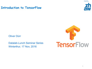
PyDNetPyDNet is a Encoder-Decoder (Autoencoder) fullyconvolutional network with a pyramidal structure: the Encoder is composed by 6 levels: each levelextract useful information (features) starting fromthe output of the previous one, and maps theminside an higher dimensionality space. the Decoder phase has to map encoder features intodepth values. It is actually made up by 6 tinydecoders.We are going to see them in details
EncoderEach level in the encoder first apply a 2D conv (in orange) with stride 2, followedby a 2D conv with stride 1 (in blue).Number of filters are respectively 16, 32, 64, 96, 128 and196 for levels from 1 to 6.We are gradually decreasing the spatial dimension of theinputs of each level (so, convolutions would be faster!)but at the same time we are increasing the number offeatures extracted.For instance, last level returns B x H/64 x W/64 x 196volumes, where B is batch size, while H and W the imageshape.
DecoderEach decoder is able to predict a depth map at a certainresolution: starting from bottom (L6), depth are estimateat 1/64, 1/32, 1/16, ⅛, ¼ and ½ of the original input.Each decoder applies 4 2D convolutions to obtain afeature volume. This volume is both convolved by a finalconv2D to obtain a depth map, and upsampled throughbilinear upsampling. The upsampled volume is given tothe next decoder in the pyramid.To restore original resolution we can apply upsamplingoperations (e.g., bilinear upsample) to depth map.
DecoderWhy multiple predictions?The key idea is that if we are using a powerful devices then we can process the fullpyramid, otherwise we can stop early!You have to find the right trade off between accuracy and computational time,depending on your application.Rgb imageHalfQuarter
What is TensorFlow TensorFlow offers API for Python, Java and C/C In this course we will use TensorFlow 1.x, even if the new version of TensorFlow called TensorFlow 2 is going to be released (but it has a different paradigm with respect to the previous version) In TensorFlow 1.x, t