Transcription
Local Economic and Political Effects of Trade Deals:Evidence from NAFTAJiwon Choi, Ilyana Kuziemko, Ebonya Washington, Gavin Wright*January 26, 2021Preliminary and incomplete. Comments welcome.AbstractWe show that counties whose 1990 employment depended on industries vulnerableto Mexican import competition via the 1994 North American Free Trade Agreement(NAFTA) suffer large employment losses (relative to the bottom quartile of counties,counties in the top quartile of NAFTA exposure see 5-8 log-point declines in employment by 2000). Despite large employment losses, we can reject even modest populationdeclines. Trade-adjustment-aid relief rises, but covers a tiny share of the job losses wedocument, and Disability Insurance in fact displays a much larger response. Exposedcounties (many in the upper South) begin the period more Democratic in terms of votesin House elections, but as NAFTA is debated in 1992-1994 they shift in the Republicandirection and by 2000 vote majority-Republican in House elections. We show with avariety of microdata, including 1992-1994 respondent-level panel data, that oppositionto free trade predicts shifts towards Republican party identification.JEL Classification Numbers: D72, F16, H5Key words: Trade agreements, Trade and labor markets, Social programs, Elections* Wethank seminar participants at Columbia, Cornell, Princeton, and Stanford. We also thankconference participants at the Labor Studies meeting at the NBER Summer Institute and theInternational Trade and Institutions conference at the NBER. David Autor, Gene Grossman, LarryKatz, Dani Rodrik and Stephen Redding provided especially helpful feedback. Paola G. VillaParo, Qianyao Ye and Arkey Barnett provided outstanding research assistance. Choi: PrincetonUniversity (email: jwchoi@princeton.edu); Kuziemko: Princeton University and NBER (email:kuziemko@princeton.edu); Washington: Yale and NBER (email: ebonya.washington@yale.edu);Wright: Stanford and NBER (email: write@stanford.edu).
1IntroductionIn September of 1993, the Clinton administration released a letter signed by 283 economists,including twelve Nobel laureates, urging Congress to ratify the North American Free TradeAgreement (NAFTA). “[T]he assertions that NAFTA will spur an exodus of U.S. jobs toMexico are without basis,” the economists wrote. “The letter is part of a concerted WhiteHouse campaign to rebut the criticisms of the trade agreement made by Texas billionaireRoss Perot, who has begun spending large amounts of his considerable fortune to promotehis view that NAFTA will destroy American jobs,” reported the Los Angeles Times.1The White House indeed succeeded in passing NAFTA in a close and bi-partisan votea few months later, and it was implemented on January 1st, 1994. However, a quarterof a century later, it remains controversial. President Donald Trump made opposition toNAFTA a key part of his successful 2016 campaign, claiming in the first presidential debatethat “NAFTA is the worst trade deal maybe ever signed anywhere, but certainly ever signedin this country.” While somewhat forgotten, as his administration was generally pro-freetrade, Senator Barack Obama campaigned against NAFTA in the 2008 Democratic primary,tying Hillary Clinton to her husband’s championing of the policy. “[T]rade deals like NAFTAship jobs overseas and force parents to compete with their teenagers to work for minimumwage at Wal-Mart. That’s what happens when the American worker doesn’t have a voice atthe negotiating table, when leaders change their positions on trade with the politics of themoment.”Economists have long argued that despite being welfare-increasing overall, free tradecreates some “losers.” However, only recently have the costs to the losers received majorattention in the literature. In particular, the important work of Autor et al. (2013) hashighlighted the large and durable negative effects to local labor markets that were exposedto Chinese import competition from 1990 to 2007.In light of its enduring political controversy and the renewed focus on the local effects oftrade agreements, we revisit NAFTA. Surprisingly, the empirical, reduced-form evidence onlocal employment effects of trade agreements and imports more generally was rather sparseuntil the recent set of papers on the “China shock.” The work on local employment effectsof NAFTA is even more limited. In contrast to the work on NAFTA that does exist, which ismuch more structural in nature, we take a simple event-study approach to the question. Weclassify communities based on the share of their 1990 (pre-NAFTA) employment in industriesthat would become exposed to Mexican imports by the terms of NAFTA. We then examine1 See“283Top Economists Back Trade Pact, Letter Shows,” Los Angeles Times, September 4,1993, -mn-31519-story.html.1
how this fixed county trait predicts economic and other outcomes each year in our sampleperiod.We begin by showing that NAFTA had a major, negative effect on employment in areasexposed to Mexican import competition. By 2000, counties in the top quartile of our measureof NAFTA exposure saw a 5-8 log point decline in total employment, relative to the bottomquartile. These losses were concentrated in manufacturing and, importantly, exhibit no pretrends from the mid 1980s to 1994. While we begin all of our analysis by showing trends withcounty year raw data, the basic shape of our event-study coefficients are unchanged as weadd a large number of controls: pre-period county-level measures (e.g., 1990 manufacturingshare of employment, 1990 share with a college degree) interacted with year fixed effects,to control flexibly for other secular changes (e.g., automation, skill biased technologicalchange) that may affect communities differentially across time; the “China shock” measurefrom Autor et al. (2013) interacted with year fixed effects, to ensure we isolate the NAFTAeffect from the rise of Chinese imports; and fixed effects at the state year level, to pick upany policy or other unobserved variation within states across time.The large employment losses might lead to population declines (as in Blanchard et al.,1992, though they examine data from an earlier period), so we examine annual populationmeasures. We find no population respond to NAFTA-driven employment losses, at least inthe medium-run captured by our sample period. We have the power to reject even smalleffects. Note that Autor et al. (2013) also find limited migration response to the Chinashock, so our result deepens the puzzle of why population does not appear to respond tothese large, trade-driven employment shocks.W examine whether DI grows in these areas from 1994 onward, given past work suggestingthat DI applications respond to local economic downturn (Autor and Duggan, 2003). Weonly have data for a subset of counties (though they capture about three-fourths of thepopulation), but at least in this subset the DI response is large and sustained—roughlyequal in percentage terms to the employment effect. We estimate that for every ten joblosses due to NAFTA in these counties, XX apply to DI. While the response in per capitaTrade Adjustment Assistance aid is statistically significant and visually detectable, it is farsmaller in magnitude: XXX.Having documented large, negative local employment effects in communities exposed toMexican import competition, we then ask how voters in these communities reacted. NAFTAwas a major issue in the 1992 U.S. presidential campaign, with Ross Perot making oppositionto it a major motivation for his third-party campaign, a third-party campaign that pickedup 19 percent of the popular vote, making it the most successful such campaign since TeddyRoosevelt’s run as the Bull Moose Party candidate in 1912. President Bill Clinton made2
passage of NAFTA a key goal of the first year of his administration, which he accomplishedvia a close, controversial and bi-partisan vote in November of 1993.We focus on House election votes in most of our political analysis, as every House seatis up for election every two years, allowing for a balanced panel of years.2 While NAFTAexposed counties (many in the upper South) begin the sample period more Democratic asmeasured by House election votes than the rest of the country, they exhibit a sharp changein trend and become increasingly Republican. In contrast to our employment effects, whichshow no pre-1994 pre-trend regardless of specification, this political turning point occursin either the 1992 or the 1994 election, depending on the controls we include in the eventstudy analysis. We find this ambiguity unsurprising, given the political salience of NAFTAin the 1992 election, even though its provisions did not go into effect until January 1994.Beyond the ambiguity between 1992 and 1994, there is no political pre-trend in NAFTAexposed counties from 1980 to 1990. The shift we document is large. While these countiesare in 1990 the most Democratic of our four quartile groups, by 2000 they are as or moreRepublican than any of the quartiles.We present a variety of microdata-based evidence that the political shift was indeeddue to NAFTA. First, we show that in the areas we define as most vulnerable to NAFTA,survey respondents significantly oppose NAFTA and this opposition continues to the presentday. Second, in repeated cross-section data from the American National Election Surveys(ANES) we show that, in each year of survey data from 1986 to 1992, Democrats enjoy asignificant and steady advantage among those with protectionist views, but between 1992and 1996 a significant number of protectionist voters move toward the GOP and remainthere. Finally, in an ANES panel dataset from 1992 to 1994, we can look at the same votersover time during this key moment. We indeed find that a significant share of those who in1992 express protectionist views have moved their party-identification toward the GOP by1994. We show these effects are robust to flexibly controlling for a variety of demographicvariables as well as views on other political and policy questions.Our paper contributes to the literature on the local employment effects in rich countriesof exposure to import competition from poorer countries. Shortly after NAFTA’s passage,Rodrik (1997) warned that academics and policy-makers were underestimating the effects ofglobalization on high-income country governments’ ability to pursue domestic policy goals.But it was not until more recently that empirical evidence on the employment effects of2 Obviously,House elections are determined by votes in Congressional Districts, which changeover time. However, data breaking down these votes into counties is readily available and we usethem so that we can examine consistent geographical unites over longer periods of time, as countyboundaries are very stable.3
trade deals gained prominence. In the U.S. context, Autor et al. (2013) highlighted the largeand lasting effects of Chinese import competition on exposed U.S. communities in terms ofdeclining employment and labor force participation and rising transfer payments.There has been limited work of this type for NAFTA. The closest is likely Hakobyanand McLaren (2016). Like Autor et al. (2013), they use Census data, so focus on longer(ten-year) differences than we do. In particular, they use decennial Census data and modelindustry-level effects of NAFTA (proxied as changes in earnings by industry from 1990 to2000) as a function of both 1990 tariff levels and the change in tariff levels between 1990and 2000.3 We bring much less structure to our empirical approach, allowing each county’s1990-level of protection to have an unrestricted effect on employment (as well as myriadother outcomes) in every year of our sample period and then plot these estimated effects.Relative to both Hakobyan and McLaren (2016) and Autor et al. (2013), our use of annualdata as opposed to Census microdata (which are available at lower frequency) allow us tovisually test for pre-trends and moreover show that breaks in trend are highly correlated intime with NAFTA’s implementation.The literature on the effect of NAFTA on the U.S. has focused on examining the policy’simpact on prices and trade flows as well as measuring its aggregate wage and welfare impact.Krueger (1999) documents the expansion of trade flows among the three North Americancountries during the first four years of NAFTA, with a potential trade diversion away fromnon-NAFTA countries. Romalis (2007) uses detailed trade flow and tariff data to estimateimport supply and demand elasticities and evaluates the price and welfare impact on theU.S. The paper finds a positive impact on the trade quantities but moderate impact on pricesand welfare. Caliendo and Parro (2014) develop a structural general equilibrium model thatincorporates the sectoral linkages (e.g., intermediate goods and input-output linkages) andshow that NAFTA had a positive impact on U.S.’s welfare by 0.08 percent, while it increasedMexico’s welfare by 1.31 percent and decreased Canada’s welfare by 0.06 percent.4It is interesting to speculate why there has been so little work on the local employmenteffects of NAFTA, and we can imagine at least two likely reasons. First, economists pushingfor its passage in the early 1990s emphasized it would have small effects. A good exam3Apotentially important issue with including both the change in tariff levels from 1990 to 2000and the level of tariff levels in 1990 is that the two are nearly one-for-one (negatively) correlated,as tariffs are mostly stable from 1990 to 1993 and then from 1994 to 2000 almost all tariffs go tozero as a result of NAFTA. Thus, identification is reliant on the relatively small share of industrieswhose tariffs with Mexico do not go to zero by 2000.4 There are papers that document the effect of NAFTA on Mexico, including Hanson (1998)that shows NAFTA affected the regional employment in Mexico by contracting manufacturingemployment in Mexico City and increasing the manufacturing employment in northern Mexico.4
ple is the public letter referenced in the first paragraph of the paper. While signatoriesacknowledged that trade deals create “winners and losers,” they stressed that the Mexicaneconomy was too small to appreciably affect U.S. employment. Second, they also emphasizedthat the provisions of NAFTA would ease tariffs downward gradually. In fact, both claimsare debatable. As we discuss in the next section, Mexican import value to the US were infact greater to that from China until 2004. Moreover, more than half of the tariffs thatexisted on Mexican goods pre-NAFTA were set to zero immediately upon the agreement’simplementation in January of 1994.5We also contribute to a small but growing literature on the political effects of tradeshocks. To date, this literature has found mixed results in the U.S. context. In a follow-upto Autor et al. (2013) work on local labor markets, Autor et al. (2016) find that voters moreimpacted by Chinese import competition move ideologically to the right on average, sendingmore polarizing representatives to Congress as voters in initially Democratic districts sendslightly more liberal candidates while voters in initially Republican districts send substantially more conservative candidates. Their findings echo papers on Germany and France thatdemonstrate that greater import competition results in a larger vote share for the far rightparty (Malgouyres (2017) and Dippel et al. (2015)). In the British case, greater exposureto trade predicts votes for Brexit (Colantone and Stanig (2018)). Che et al. (2017), on theother hand, using a longer time period (1990 to 2010 where Autor et al. (2016) examine2002-2010) level of geography (counties, which stay constant over a 20 year period as opposed to districts) and methodological approach (focusing on a policy change that resultedin greater Chinese import competition for some areas) than Autor et al. (2016) find that themost exposed to Chinese imports are more likely to vote Democratic.By contrast with the literature on the political response to the China shock, we find aclear shift in the Republican direction in places most exposed to NAFTA and among votersopposed to free trade. We suspect that the difference lies in the political saliency of NAFTA.The debate over NAFTA motivated a highly successful third-party presidential campaign in1992 and remains a politically controversial point to this day. As we discuss in Section 6,NAFTA captured much more attention on network nightly news than did the later easing oftrade relations with China. Why NAFTA captured media and public attention more thandid easing of trade relations with China is an interesting question for future work.The rest of the paper is organized as follows. Section 2 provides a short background onNAFTA’s provisions and describes how we measure local vulnerability to NAFTA. Section 35 SeeU.S. Information Agency (1998), p. 25. Also, our documentation of tariff protection byyear in the next section shows a large and immediate decline in tariff rates in 1994 and 1995, andthen a slower convergence thereafter to zero.5
outlines the empirical strategy for our event-study analysis. Section 4 describes the employment results, Section 5, the demographic and transfer-program results and Sections 6 and 7the political results. Section 8 concludes and offers ideas for future work.2Measuring local vulnerability to NAFTA2.1Background on the agreementBy 1992, diplomats from Canada, Mexico and the US had hammered out the details of anhistoric agreement to substantially reduce trade barriers across the North American continent, though the agreement awaited ratification by the governments of the three countries.In fact, trade between the US and Canada had mostly been tariff-free due to earlier agreements, so the debate over NAFTA in the US focused on whether to liberalize trade withMexico.As noted in the introduction and discussed in greater detail in Section 6, NAFTA becamea major issue in the 1992 election in the US. President Clinton eventually secured its passagein November 1993, and many of its provisions went into effect in January 1994. WhileNAFTA phased out some tariffs more gradually, in fact over one-half of tariffs on Mexicangoods were immediately set to zero in 1994.Figure 1 shows the value of imports to the US from Mexico (and, for context, also includesChina). While growing before NAFTA, Mexican imports enjoy more rapid growth beginningin 1994. Interestingly, despite the larger focus on China in the empirical labor economicsliterature, it is not until 2004 that China supplants Mexico as the most important lowincome source of imports (though its rise since 2004 is indeed more rapid than any periodfor Mexico).Which industries were most affected by NAFTA? Not surprising given Mexico’s comparative advantage in low-skilled labor, they were labor-intensive, low-wage manufacturingindustries such as apparel, shoes, textiles and leather. It is important to note that theseindustries had long complained about import competition from poor countries and weredeclining even before NAFTA and the China Shock.6 In fact, industry lobbyists often complained about an assumption among politicians and economists that these jobs were in“sunset industries” and moreover were low-quality jobs that were not worth saving. But atthe time of NAFTA’s passage, the apparel and textile industries still employed nearly twomillion people. Whether via a successful (at least in terms of visibility) “Made-in-America”6 Muchof the information provided in this paragraph is taken from Minchin (2012a), a historyof the decline of the U.S. textile industry.6
campaign pitched toward consumers or other factors, employment decline had also slowedin these industries in the years leading up to NAFTA. We show in Appendix Figure A.1that employment in textile mills was in fact quite stable in the early 1990s (at half a millionworkers) before beginning a rapid decline in the middle of the decade.2.2Construction of our measure of NAFTA exposureOur exposure measure draws heavily from Hakobyan and McLaren (2016), though we createcounty-level measures, whereas they examine exposure at the Public-Use Micro-data Area(PUMA) level. In spirit, it is also very similar to that used by Autor et al. (2013), as ittakes the vector of industry-level measures of exposure to import competition and, for eachcommunity, multiplies it by a vector of pre-period industry employment shares.Following Hakobyan and McLaren (2016), we begin by creating Mexico’s “relative comparative advantage” (RCA) in a given industry j I, using 1990 (pre-NAFTA) data: ROWEXxMj,1990 /xj,1990RCA P M EX P ROW .i xi,1990 /i xi,1990j(1)EXIn the numerator of the above expression, xMj,1990 is the 1990 value of Mexican exports (to allcountries, not just the US) in industry j, xROWj,1990 is the 1990 value of the rest of the world’s(ROW) exports (again, to all countries) in j. The ratio of the two expressions is roughlyequal to Mexico’s share of exports in industry j. Of course, the share will be in part drivenby Mexico’s size. The denominator adjusts for Mexico’s overall share of all exports, not justthose in industry j. Thus, the overall expression in equation (1) captures, in 1990, Mexico’srelative advantage in producing exports in industry j relative to other industries i I.Because we use so many different data sources in this paper (and many of them are wellknown to economists) we do not have a separate data section and instead in the interest ofspace briefly describe the data we use in each section and refer readers to Appendix B formore detail. We use data from XXX to calculate the the RCA for each industry j.How much a U.S. county is likely to be affected by NAFTA depends on its pre-periodreliance on employment from industries with the following two characteristics: (a) Mexicohas large RCA in that industry, and (b) the industry had previously enjoyed tariff protectionbefore NAFTA.We can now write our full county-level vulnerability measure:PJcjj jj 1 L1990 RCA τ1990,PJcjjLRCAj 1 1990Vulnerabilityc,1990 7(2)
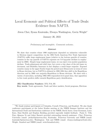
jwhere Lcj1990 is employment of industry j in county c in year 1990 and τ1990 is the ad-valoremequivalent tariff rate of industry j in 1990. Note that the measure uses only pre-periodmeasures of both Mexican RCA and community-level industrial composition, and thus doesnot pick up any endogenous reaction to NAFTA itself. County-level employment data comefrom XXX and tariff data from XXX.There are three conceptual points to discuss about the vulnerability expression in equation (2). First, it is a constant within county—as we take the τ j values from 1990, it captureshow much tariff protection from Mexican RCA a county enjoyed in 1990. The event-studyspecification asks what predictive value this county-level constant has in each year of thesample period.jOf course, while our τ1990are taken from a specific year, the τ j values in fact change overtime, in particular a large decline in the mid-1990s due to NAFTA. Figure 2 shows, separatelyby quartile of 1990 vulnerability, how the protection measure in equation (2) changes if weallow the τ to follow their actual course over time (all other variables in the expression arekept at their 1990 levels, so the value of the four series in 1990 is in fact the average countyvulnerability measure, as defined in equation 2, for the four groups). Before 1993, there islittle change, as tariff rates were largely stable in this pre-NAFTA period. Between 1993and 1995, there is a large decline in protection, consistent with NAFTA setting the majorityof tariffs to zero within the first year. By 2000, even the most protected quartile of countiesby the 1990 measure have essentially zero tariff protection.Second, as there is little change in tariffs between 1990 and 1993, and between 1994 and2000 most tariffs go to zero, there is an extremely high correlation between 1990 tariffs andthe 1990 to 2000 change in tariffs. Thus, “protection” from Mexican import competition in1990 is essentially the same as “vulnerability” or “exposure” to NAFTA and we use theseexpressions interchangeably.Third, while similar in spirit to the ADH measure, one departure is that we focus onstatutory changes in tariff protection instead of changes in actual import penetration. Weview this modification as somewhat preferable, as actual imports are potentially endogenousto domestic demand (Autor et al., 2013 themselves note this concern, and thus use Chineseimport flows to other rich countries as an instrumental variable in many specifications).In principle, tariff reductions could have a direct effect on local employment without anactual rise in Mexican imports in once-protected industries: the announcement of the tariffreductions themselves could deter future investment in those domestic industries and thusreduce employment. But in practice, Mexican imports in once-protected industries indeeddid rise after NAFTA. Appendix Figure A.2 shows the value of three different groups ofMexican imports to the US from 1990 to 2000: those with no tariff protection in 1990 and8
then two groups of industries who enjoyed some protection in 1990 (split at the median 1990tariff level). While the first group shows no change upon NAFTA’s implementation, the othergroups do, with a larger effect for those industries enjoying greater levels of protection in1990. Thus, higher 1990 tariff levels for a given industry does indeed predict larger increasesin Mexican imports post-NAFTA.2.3Geographic variation in the NAFTA exposure measureWhile Figure 2 shows how tariff protection changed over time, Figure 3 shows how protectionin 1990 (and thus vulnerability to NAFTA) varies geographically. The upper South exhibitsthe highest levels of vulnerability, but there are pockets of high-vulnerability areas withinmost states.A natural question is how our measure of NAFTA vulnerability varies with exposure tothe China shock in Autor et al. (2013). Many of the same industries were affected (textilesand apparel, e.g.). However, the correspondence is hardly one-for-one. At the CZ level, the(1990 population-weighted) correlation is 0.172. As noted, ADH often use an instrumentedversion of their exposure measure, and the correlation in that case is 0.420. Thus, whilepositively correlated, they are not identical, though in all of our analysis we show resultsafter flexibly controlling for the China-shock measures.2.4Characteristics of counties by NAFTA vulnerabilityTable A shows a variety of county-level summary statistics, separately by quartile of NAFTAexposure. In terms of size, the most and least exposed quartiles are the most similar, bothhaving few people, workers and firms than the second and third quartiles.Individuals in our most exposed quartile begin our sample period the most reliant onmanufacturing employment and the least likely to have a college degree, highlighting theimportance of flexibly controlling for these attributes in order to isolate the effects of NAFTAfrom secular changes such as skill-biased technological change or the China shock that couldalso disproportionately hurt these areas.As the most vulnerable quartile is disproportionately Southern, it is not surprising that itis less white than the other quartiles, as African-Americans have always disproportionatelylived in the South. It also begins the period the least supportive of Republican candidates in House elections. While the South was no longer a Democratic stronghold by 1990,Democrats, in part because of their senior positions in Congress, still faired well in Houseand Senate elections in the region.77 SeeKuziemko and Washington (2018) on the decline of Democratic party identification among9
3Empirical strategy for event-study analysisEvent-study analyses provide the bulk of the evidence in this paper (an exception beingsome of the political results in Sections 6 and 7). Indeed, we view as one of our contributions relative to the existing literature on local employment effects of trade agreements isthat we present results in a very simple and transparent manner, which allows readers toeasily inspect pre-NAFTA trends and to determine if any changes are coincident with theimplementation of the agreement.We generally begin by showing trends for four groups of counties: the four quartilesas defined by the NAFTA vulnerability measure. These trends are based on raw data,unadjusted except for normalization of each quartile to zero at 1993. While this approachis the most transparent, it is more difficult to summarize and to adjust for covariates ina concise manner. We thus turn to a standard event-study approach for the bulk of ouranalysis, where instead dividing NAFTA exposure into quartiles we simply use (linearly) themeasure in equation (2), interacting it with year fixed effects. In particular, we estimate:Yct αc γt X βt Vulnerabilityc,1990 1 t t̃ λXct ct ,(3)t̃6 1993where Yct is a given outcome in county c in year t (employment, population, etc.); αc arecounty fixed effects; γt are year fixed effects, Vulnerabilityc,1990 is the vulnerability index in c(measured, as discussed in the previous section, using data from 1990); Xct include controlsthat vary within community over time (which we vary to probe robustness); and ct is theerror term. The exact sample period depends on the outcome variable and data availability,but in general we begin in the late 1980s and end in the early 2000s. We cluster standarderrors at the state level.Note that this equation does not directly use the schedule of tariff reductions implied byNAFTA (and plotted earlier in Figure 2). Instead, we allow the 1990 level of tariff protectionto have an unrestricted effect in each year, captured by the βt coefficients, and plot thoseestimated effects each year. We prefer to take a more agnostic approach to how the ef
that \NAFTA is the worst trade deal maybe ever signed anywhere, but certainly ever signed in this country." While somewhat forgotten, as his administration was generally pro-free-trade, Senator Barack Obama campaigned against NAFTA in the 2008 Democratic primary, tying Hi