Transcription
Unit 7Relationships in Data
Topic 26Graphical Displays of AssociationIn-Class ActivitiesActivity 26-5: Heights, Handspans, and Foot Lengths26-5, 28-1, 29-12, 29-13, 29-14You will use SPSS in parts a, b, and c of this activity.a. Use SPSS to create a scatterplot of height vs. handspan. Do these variables appear tobe associated? If so, describe the association in your main textbook?1. Enter the data in SPSS. See Activity 2-1 for instructions on entering new data.Create one variable for the height data, another for the handspan data, and a thirdfor the gender data. Be sure that gender is a nominal variable, and create valuelabels. To check or change the data type, use the Measure column in theVariable View tab.2. Select Graphs Chart Builder to bring up the dialog box shown below.3. From the Gallery select Scatter/Dot, and drag the picture of the simplescatterplot (the one in the upper left corner) to the Chart preview box.4. Drag the response variable (Height) to the Y-Axis? box and drag the explanatoryvariable (Handspan) to the X-Axis? box5. Click OK to create the plot.
b. Use SPSS to create a labeled scatterplot of height vs. handspan, using different labelsfor men and women. Use the graph to comment on the three questions posed in yourmain textbook.1. Select Graphs Chart Builder to bring up the dialog box shown below.2. From the Gallery select Scatter/Dot, and drag the picture of the scatterplot withdifferent colored circles to the Chart preview box.3. Drag the response variable (Height) to the Y-Axis? box and drag the explanatoryvariable (Handspan) to the X-Axis? box. Drag the group-identifying variable(Gender) to the Set color box.4. Click OK to create the graph.
c. Use SPSS to create scatterplots and conduct a similar analysis of height vs. footlength, describing the relationship between them and comparing that relationshipbetween the two sexes.Activity 26-6: Televisions and Life Expectancy26-6, 27-3, 28-19You will use SPSS to create the requested scatterplot in part b of this activity. Completeall other parts as directed in your main textbook.b. Use SPSS to produce a scatterplot of life expectancy vs. televisions per thousandpeople. The data are stored in the SPSS file TVlife06.SAV. Does there appear tobe an association between the two variables? If so, describe its direction, strength,and form. See Activity 26-5 for instructions on creating scatterplots.\
Activity 26-7: Kentucky Derby TimesYou will use SPSS in parts b and c of this activity. Complete all other parts as directed inyour main textbook.b. Use SPSS to create the requested histogram. The data are stored in the SPSS fileKYDerby.SAV.c. Use SPSS to create the requested scatterplot.ExercisesExercise 26-9: Challenger Disaster26-9, 27-17Use SPSS to create the scatterplots requested in parts a and d of this exercise. The dataare stored in the SPSS file Challenger.SAV.Exercise 26-11: Broadway Shows2-14, 26-10, 26-11, 27-15Use SPSS to produce the labeled scatterplot requested in part a. The data are stored inthe SPSS file Broadway06.SAV.Exercise 26-14: Fast Food Sandwiches26-14, 26-15, 28-16Use SPSS to create the scatterplot requested in part a and to create the labeled scatterplotrequested in part b. The data are stored in the SPSS file Arbys06.SAV.Exercise 26-15: Fast Food Sandwiches26-14, 26-15, 28-16Use SPSS to produce the requested scatterplots. The data are stored in the SPSS fileArbys06.SAV.
Exercise 26-16: College Alumni Donations26-16, 27-16Use SPSS to analyze the distribution donor percentages requested in part a. Use SPSS toproduce the scatterplots requested in parts c and d. The data are stored in the SPSS fileHMCDonors.SAV.Exercise 26-17: Peanut ButterUse SPSS to produce the scatterplot requested in part c and to produce the labeledscatterplot request in part d. The data are stored in the SPSS file PeanutButter.SAV.Exercise 26-21: Comparison Shopping23-22, 23-23, Lab 6, 26-21Use SPSS to create the scatterplot requested in part b. The data are stored in the SPSSfile Shopping.SAV.Exercise 26-24: Word Twist23-24, 23-25, 26-24, 28-27Use SPSS to produce the scatterplot requested in part b. The data are stored in the SPSSfile WordTwist.SAV.Exercise 26-26: Cat Jumping26-26, 26-27, 28-29, 28-30, 29-20Use SPSS to produce the scatterplots requested in part a. The data are stored in the SPSSfile CatJumping.SAV.Exercise 26-27: Cat Jumping26-26, 26-27, 28-29, 28-30, 29-20Use SPSS to produce the labeled scatterplot requested in part a and to produce thecomparative dotplots requested in part b. The data are stored in the SPSS fileCatJumping.SAV.
Exercise 26-30: Life Expectancy26-29, 26-30, 28-34, 28-35Use SPSS to produce the scatterplots requested in part a. The data are stored in the SPSSfile LifeExpectancy2008.SAV.Exercise 26-32: Scrabble Names26-32, 29-23Use SPSS to produce the scatterplot requested in part a, to create the new variable anddotplot requested in part g, and to produce the scatterplot requested in part h. The dataare stored in the SPSS file ScrabbleNames.SAV.Exercise 26-33: Airline MaintenanceEnter the data into SPSS and use SPSS to produce the scatterplot requested in part b.
Topic 27Correlation CoefficientIn-Class ActivitiesActivity 27-1: Car Data26-3, 27-1, 28-10You will use SPSS in parts a and b of this activity. Complete parts c—f as directed inyour main textbook.a. Use SPSS to calculate the value of the correlation coefficient between time to travel¼ mile and weight. Record this value in the table on page 594 of your main textbookin the column corresponding to scatterplot A.1. Open the SPSS data file Cars99.SAV.2. Select Analyze Correlate Bivariate to open the dialog box shown below.3.Enter the two variables whose correlation coefficient you want in the Variablesbox.4. Make sure that Pearson is checked in the Correlation Coefficients area5. Click OK. A table like the one shown below will be produced in an Outputwindow. From it you will se that the desired correlation coefficient is r -0.450.Record this value in the table on page 594 of your main textbook under the letterA shown there.
b. Now use SPSS to calculate the value of the correlation coefficient for the other eightscatterplots. Record these values in the table on page 594 of your main textbookbelow the appropriate letters.Activity 27-2: Governors’ SalariesYou will use SPSS in parts b, d, and f—h of this activity. Complete all other parts asdirected in your main textbook.b. Use SPSS to produce a scatterplot of governor’s salary vs. median housing price.The data are stored in the SPSS file Governors08.SAV. Describe the association(direction, strength, and form) between these two variables. See Activity 26-5 forinstructions for producing scatterplots.d. Use SPSS to calculate the value of this correlation. Record this value in your maintextbook and comment on the accuracy of your guess. See Activity 27-1 forinstructions on calculating correlations.f. Suppose Hawaii gives its governor a 100,000 raise. Make this change in the data.Then reproduce the scatterplot and recalculate the value of the correlation coefficient.Has the correlation coefficient changed much?g. Repeat part f, after giving the governor of Hawaii an additional 100,000.h. Return Hawaii to its original value. Now change California’s governor’s salary to 0.(Former governor Schwarzenegger waived his salary as governor.) Then reproducethe scatterplot and recalculate the correlation coefficient. Has the correlationcoefficient changed much?Activity 27-3: Televisions and Life Expectancy26-6, 27-3, 28-19You will use SPSS in part c of this activity.c. Use SPSS to calculate this correlation coefficient. The data are stored in the SPSSfile TVlife06.SAV. How accurate was your guess. See Activity 27-1 forinstruction on calculating correlations. Record you value in your main textbook.
Activity 27-5: Housing Prices19-22, 26-1, 27-5, 27-25, 28-2, 28-12, 28-13, 29-3You will use SPSS in part d of this activity.d. Confirm your calculation in part b by using SPSS to calculate the value of thecorrelation coefficient between house price and size. The data are stored in the SPSSfile HousePricesAG.SAV. See Activity 27-1 for instructions on calculatingcorrelations.Activity 27-6: Exam Score Improvements23-19, 23-20, 23-21, 27-6You will use SPSS in parts a, b, d, f, h, and j of this activity.a. Use SPSS to produce a scatterplot of exam 2 score vs. exam 1 score. The data arestored in the SPSS file ExamScores.SAV. Comment on the direction, strength,and form of the association. See Activity 26-5 for instructions on creatingscatterplots.b. Use SPSS to calculate the correlation coefficient between exam 2 score and exam 1score. See Activity 27-1 for instructions on calculating correlations.d. Use SPSS to make this change (subtract 10 points from every score on exam 1). UseTransform Compute Variable. Reproduce the scatterplot of exam 2 score vs. newexam 1 score and recalculate the correlation coefficient. How did the correlationvalue change?f. Use SPSS to make this change: double everyone’s score on exam 2. Reproduce thescatterplot of new exam 2 score vs. exam 1 score and recalculate the correlation.How did the correlation value change?h. Make up some hypothetical bivariate data with the property described in part g. Hint:Choose any values for the exam 1 scores, and then make sure each exam 2 score is 10points higher. Do this for at least 5 hypothetical students. Then use SPSS to producea scatterplot and calculate the correlation coefficient. Does this confirm the value youexpected in part g or do you need to revise your thinking?j. Make up some hypothetical bivariate data with the property described in part i. Thenuse SPSS to produce a scatterplot and calculate the correlation coefficient. Does thisconfirm the value you expected in part I or do you need to revise your thinking?
Activity 27-7: Draft Lottery10-18, 27-7, 29-9You will use SPSS in parts c—e of this activity.c. Use SPSS to produce a scatterplot of draft number vs. sequential data of the birthday.The data are stored in the SPSS file DraftLottery.SAV. Based on thescatterplot, guess the value of the correlation coefficient. Explain the reasoningbehind your guess. See Activity 26-5 for instructions on creating scatterplots.d. Use SPSS to calculate the value of the correlation coefficient. Does the valuesurprise you? If so, look back at the scatterplot to see whether, in hindsight, its valuemakes sense. Summarize what the value of this correlation coefficient reveals abouthow the draft numbers were distributed across birthdays throughout the year. SeeActivity 27-1 for instructions on calculating correlations.e. Data for 1971 are also stored in the SPSS file DraftLottery.SAV. Examine ascatterplot and calculate the correlation coefficient between draft number andsequential date for that year’s lottery. Comment on your findings in your maintextbook.ExercisesExercise 27-8: Hypothetical Exam Scores7-12, 8-22, 8-23, 9-22, 10-22, 27-8Use SPSS to calculate the correlation coefficients requested in parts c and f. The data arestored in the SPSS file HypoExams.SAV.Exercise 27-10: Monopoly27-10, 27-11Use SPSS to produce the scatterplots and calculate the correlation coefficients requestedin parts a, b, and c. The data are stored in the SPSS file Monopoly.SAV.Exercise 27-10: Monopoly27-10, 27-11Use SPSS to calculate the correlation coefficients requested in parts d and f. The data arestored in the SPSS file Monopoly.SAV.
Exercise 27-12: Monthly Temperatures9-26, 26-12, 27-12Enter the data into SPSS and use SPSS to calculate the correlation coefficient requestedin part b.Exercise 27-15: Broadway Shows2-14, 26-10, 26-22, 27-15Use SPSS to calculate the correlation coefficients requested in part a. The data are storedin the SPSS file Broadway06.SAV.Exercise 27-16: College Alumni Donations26-16, 27-16Use SPSS to produce the scatterplots requested in part a and to calculate the correlationcoefficients requested in parts b and e.Exercise 27-17: Challenger26-9, 27-17Use SPSS to calculate the correlation coefficients that are requested. The data are storedin the SPSS file Challenger.SAV.Exercise 27-18: Solitaire11-22, 11-23, 13-12, 15-3, 21-20, 27-18Use SPSS to produce the requested scatterplots and calculate the requested correlationcoefficients. The data are stored in the SPSS file Solitaire.SAV.Exercise 27-19: Climatic ConditionsUse SPSS to calculate the requested correlation coefficients. The data are stored in theSPSS file Climate.SAV.Exercise 27-20: Muscle Fatigue23-2, 23-27, 23-28, 26-22, 27-20Enter the data into SPSS and use SPSS to calculate the correlation coefficient in part a.
Exercise 27-21: Digital Cameras10-5, 26-18, 27-21Use SPSS to calculate the correlation coefficients requested in parts a and b. The data arestored in the SPSS file DigitalCameras.SAV.Exercise 27-24: Utility Usage26-28, 27-24, 28-28, 29-21Use SPSS to calculate the correlation coefficients requested in part b. The data are storedin the SPSS file Utilities.SAV.Exercise 27-25: House Prices19-22, 26-1, 27-5, 27-25, 28-2, 28-12, 28-13, 29-3Use SPSS to calculate the correlation coefficients requested in parts a and b. The data arestored in the SPSS file HousePricesAG.SAV.Exercise 27-26: Kentucky Derby26-7, 27-26, 27-27, 27-28, 28-32, 28-33Use SPSS to calculate the correlation coefficient requested in part a. Use SPSS to createthe new variable Winning Speed and to produce the scatterplot and calculate thecorrelation between it and year as requested in part c. The data are stored in the SPSSfile KYDerby.SAV.Exercise 27-27: Kentucky Derby26-7, 27-26, 27-27, 27-28, 28-32, 28-33Use SPSS to create the new variable Winning Speed and to produce the histogramrequested in part a. Use SPSS to produce the scatterplot and calculate the correlationcoefficient requested in part b. The data are stored in the SPSS file KYDerby.SAV.Exercise 27-28: Kentucky Derby26-7, 27-26, 27-27, 27-28, 28-32, 28-33Use SPSS to calculate the correlation coefficients requested in parts a and b. The data arestored in the SPSS file KYDerby.SAV.
Topic 28Least Squares RegressionIn-Class ActivitiesActivity 28-2: House Prices19-22, 26-1, 27-5, 27-25, 28-2, 28-12, 28-13, 29-3You will use SPSS in part c of this activity. Complete all other parts as directed in yourmain textbook.c. Use SPSS to confirm you calculation of the least squares line. Hint: Do not besurprised if the coefficients differ a bit based on rounding discrepancies.1. Open the SPSS data file HousePricesAG.SAV.2. Select Analyze Regression Linear to open the dialog box shown below.3. Enter the explanatory variable (Size) in the Independent(s) box, and enter theresponse variable (Price) in the Dependent box.4. Click OK.The output contains, among other things, The Coefficients and Model Summary tablesshown below. The value in the B column of the Coefficients table in the (Constant)row is the value of the intercept, a. The value in the B column in the row with the
explanatory variable is the value of the slope, b. The value in the R Square column ofthe Model Summary table is the coefficient of determination, r 2 .Activity 28-3: Animal Trotting SpeedsYou will use SPSS in parts d—g of this activity.d. Use SPSS to produce a residual plot of residuals vs. body mass for these data.1. Open the SPSS data file TrotSpeeds.SAV.2. Select Analyze Regression Linear and make body mass the independentvariable and trot speed the dependent variable. Click Save to open the dialog boxshown below.3. In the Residuals area check Unstandardized. Click Continue followed by OK.This will run the regression. A new variable, Res 1, will be created in the Dataview that contains the residuals.
4. Produce a scatterplot with the residuals on the vertical axis and body mass on thehorizontal axis. See Activity 26-5 for instructions on producing scatterplots.e. Use SPSS to take the logarithm (base 10) of the body mass variable.1. Select Transform Compute Variable to open the dialog box shown below.2. Make the target variable log body mass.3. Select Arithmetic from the Function group menu. Lg10 computes the base 10logarithm. Double click it. Lg10(?) will appear in the Numeric Expression box.Replace the question mark with the body mass variable. The dialog box shouldlook like that shown below.4. Click OK to create the new variable.
f. Use SPSS to determine the least squares line for predicting trot speed from log(bodymass). Also produce a scatterplot with this line draw on it. Record the equation ofthis line and the value of r 2 in your main textbook. Proceed as directed below toproduce this plot. Such a plot is know as a fitted line plot. You will need to selectAnalyze Regression Linear to get the equation of the least squares line.1. Select Graphs Chart Builder and create a scatterplot of trot speed vs. log(bodymass). See Activity 26-5 for instructions.2. Double click the resulting graph to open the Chart Editor shown below.3. Click the Add Fit Line at Total icon. It is the fifth icon from the left in the rowimmediately above the graph window.4. Close the Chart Editor and the scatterplot with the regression line drawn in it willreplace the original scatterplot in the Output window.
g. Use SPSS to produce a residual plot for the least squares line in part f. Does this plotreveal a random scattering of points, indicating that the linear is reasonable for thetransformed data?Activity 28-4: Textbook Prices7-29, 28-4, 28-5, 29-5You will use SPSS in parts b, d, and h—j of this self-check activity. The data are storedin the SPSS file TextbookPrices.SAV.b. Use SPSS to examine scatterplots of price vs. pages and price vs. year. Comment onwhat these graphs reveal about the association between price and these othervariables. See Activity 26-5 for instructions on scatterplots.d. Use SPSS to determine the least squares line for predicting a textbook’s price basedon its number of pages. Report the equation of this regression line, and draw the lineon the scatterplot. Hint: Be sure to use good statistical notation in report thisequation. See Activity 28-2 for instructions.h. Use SPSS to create and comment on a residual plot for this least squares line.
i. Use SPSS to determine the least squares line for predicting a textbook’s price basedon its year of publication. Report the equation of this regression line and the value ofr2 .j. Create a residual plot for this least squares line. Comment on what it reveals abouthow well the linear model summarizes the relationship between price and year. SeeActivity 28-3 for instructions.ExercisesExercise 28-6: Airfares28-6, 28-7, 28-8, 28-9, 29-16Use SPSS to create the scatterplot requested in part b. The data are stored in the SPSSfile Airfares.SAV.Exercise 28-7: Airfares28-6, 28-7, 28-8, 28-9, 29-16Use SPSS to create the residual plot requested in part c. The data are stored in the SPSSfile Airfares.SAV.Exercise 28-8: Airfares28-6, 28-7, 28-8, 28-9, 29-16Use SPSS to calculate the least squares lines and values of r 2 requested in parts b, d, ande. The data are stored in the SPSS file Airfares.SAV.Exercise 28-11: Electricity BillsUse SPSS to create the dotplot requested in part a and produce the scatterplot requestedin part b. The data are stored in the SPSS file ElectricBill.SAV.Exercise 28-12: House Prices19-22, 26-1, 27-5, 27-25, 28-2, 28-12, 28-13, 29-3Use SPSS to calculate the regression line and the value of r 2 requested in part b. Thedata are stored in the SPSS file HousePricesAG.SAV.
Exercise 28-13: House Prices19-22, 26-1, 27-5, 27-25, 28-2, 28-12, 28-13, 29-3Use SPSS to create the graphical and numerical summaries requested in part a, producethe scatterplot requested in part b, calculate the regression line and the value ofr 2 requested in part c, and produce the residual plot requested in part d. Also use SPSS toperform the analyses requested in part e. The data are stored in the SPSS fileHousePricesAG.SAV.Exercise 28-14: Honda Prices7-10, 10-19, 12-21, 28-14, 28-15, 29-10, 29-11Use SPSS to produce the scatterplot requested in part a, calculate the regression linerequested in part b, calculate the value of r 2 requested in part d, and perform the analysesrequested in part f. The data are stored in the SPSS file HondaPrices.SAV.Exercise 28-15: Honda Prices7-10, 10-19, 12-21, 28-14, 28-15, 29-10, 29-11Redo the previous exercise with manufacture as the explanatory variable. Use SPSS toproduce the scatterplot requested in part a, calculate the regression line requested in partb, calculate the value of r 2 requested in part d, and perform the analyses requested in partf. The data are stored in the SPSS file HondaPrices.SAV.Exercise 28-16: Fast Food Sandwiches26-14, 26-15, 28-16Use SPSS to produce the scatterplot requested in part a, calculate the equation of theregression line and the value of r 2 requested in part b, and produce the residual plotrequested in part c. The data are stored in the SPSS file Arbys06.SAV.Exercise 28-17: Box Office Blockbusters28-17, 28-18Use SPSS to conduct the requested full regression analysis. The data are stored in theSPSS file BoxOffice05.SAV.
Exercise 28-18: Box Office Blockbusters28-17, 28-18Use SPSS to conduct the requested full regression analysis. The data are stored in theSPSS file BoxOffice05.SAV.Exercise 28-19: Televisions and Life Expectancy26-6, 27-3, 28-19Use SPSS to produce the scatterplot requested in part a and to compute thetransformations and create the scatterplots requested in parts b and c. The data are storedin the SPSS file TVlife05.SAV.Exercise 28-20: Planetary Measurements8-12, 10-20, 19-20, 27-13, 28-20, 28-21Use SPSS produce the scatterplot requested in part a, calculate the regression equationand produce the residual plot requested in part b, calculate the transformations andproduce the scatterplots requested in part c, calculate the regression equation and thevalue of r 2 requested in part d, and produce the residual plot requested in part f. Thedata are stored in the SPSS file Planets.SAV.Exercise 28-21: Planetary Measurements8-12, 10-20, 19-20, 27-13, 28-20, 28-21Use SPSS produce the scatterplot requested in part a, compute the transformationrequested in part b, calculate the transformations and produce the scatterplots requestedin part c, calculate the regression equation requested in part d, and produce the residualplot requested in part e. The data are stored in the SPSS file Planets.SAV.Exercise 28-22: Gestation and Longevity28-22, 28-23Use SPSS to produce the scatterplot requested in part a, calculate the regression equationand the value of r 2 requested in part b, produce the residual plot requested in part d, andproduce the scatterplots and calculate the regression equations and the values of r 2 andproduce the residual plots requested in parts g and h. The data are stored in the SPSS fileGestation06.SAV.
Exercise 28-23: Gestation and Longevity28-22, 28-23Use SPSS to reproduce the regression equation to be used in part a. The data are storedin the SPSS file Gestation06.SAV.Exercise 28-27: Word Twist23-24, 23-25, 26-24, 28-27Use SPSS to produce the fitted line plot, calculate the regression line, and store theresiduals requested in pert a. The data are stored in the SPSS file WordTwist.SAV.Exercise 28-28: Utility Usage26-28, 27-24, 28-28, 29-21Use SPSS to calculate the equation of the regression line and the value of r 2 requested inpart a, and produce the residual plot requested in part d. The data are stored in the SPSSfile Utilities.SAV.Exercise 28-29: Cat Jumping26-26, 28-29, 28-30, 29-20Use SPSS to calculate the equation of the regression and the value of r 2 requested in parta, and produce the residual plot requested in part d. The data are stored in the SPSS fileCatJumping.SAV.Exercise 28-30: Cat Jumping26-26, 28-29, 28-30, 29-20Use SPSS to compute the requested new variable and perform the requested fullregression analysis. The data are stored in the SPSS file CatJumping.SAV.Exercise 28-33: Kentucky Derby26-7, 27-26, 27-27, 27-28, 28-32, 28-33Use SPSS to split the file and calculate the equation of the regression lines requested inpart a, and produce the residual plots requested in part b. The data are stored in the SPSSfile KYDerby.SAV.
Exercise 28-34: Life Expectancy26-29, 26-30, 28-34, 28-35Use SPSS to produce the scatterplots requested in part a, and calculate the equation of theregression line and the value of r 2 requested in part b. The data are stored in the SPSSfile LifeExpectancy2008.SAV.Exercise 28-35: Life Expectancy26-29, 26-30, 28-34, 28-35Use SPSS to perform the requested log transformations and produce the scatterplots andcalculate the equation of the regression lines. The data are stored in the SPSS fileLifeExpectancy2008.SAV.Exercise 28-36: Governors’ Salaries27-2, 28-36Use SPSS to produce the fitted line plot and calculate the equation of the regression linerequested in part a, and calculate the equation of the regression line requested in part c.The data are stored in the SPSS file Governors08.SAV.
Topic 29Inference for Correlation and RegressionIn-Class ActivitiesActivity 29-1: Studying and Grades29-1, 29-2, 29-7, 29-8You will use SPSS in parts b, c, n, o, p, and r of this activity. Complete all other parts asdirected.b. Open the SPSS file UOPgpa.SAV and use SPSS to construct a scatterplot of GPA vs.study hours. Describe any association revealed by the scatterplot. Is the associationwhat your expected? Explain. See Activity 26-5 for instructions on generatingscatterplots.c. Use SPSS to determine the equation of the least squares line for predicting GPA fromstudy hours, being sure to write it in the context of these two variables. See Activity28-2 for instructions on least squares.n. The table shown below is part of the standard output from SPSS for this regression.You have already seen in Topic 28 how to get the sample slope and intercept. In theB column of the Unstandardized Coefficients column, you see that a 2.886 and b .089. This table also gives the standard errors for both a and b. They are in the Std.Error column in the Unstandardized Coefficients column. Thus, SE(a) .120 andSE(b) .028. Is this reasonably close to the standard deviation of your 100 simulatedslope coefficients?o. Use the standard error from part n to calculate (by hand) the test statistic for testingwhether the population slope differs from zero. Does this value agree with the valueshown in the t column of the table shown above in the Study Hours per Week row?p. Use the t-Distribution Critical Values table (Table III) and your test statistic in part oto determine (as best you can) the p-value of the test. Is this p-value consistent withthe value shown in the Sig. column of the table shown above in the Study Hours perWeek row? The value in the table is the exact p-value for testingH 0 : 0 vs. H a : 0. Is this p-value consistent with your simulation results?Explain. If you want to run a one-sided test using SPSS results, you need to adjustthe Sig. value as shown in the table below.
Ha : 0Ha : 0IfIfIfIft 0 : p-value Sig./2t 0 : p-value 1 – Sig./2t 0 : p-value 1 – Sig./2t 0 : p-value Sig./2Use the sample slope and its standard error to form a 95% confidence interval forthe population slope coefficient. SPSS also calculated confidence intervals for theslope coefficient and intercept.1. Select Analyze Regression Linear, set up the regression, and click Statisticsto bring up the dialog box shown below.2. Check Confidence intervals in the Regression Coefficient area. Enter thedesired confidence level, as a percent, in the Level (%) box.3. Click Continue and then OK to run the regression. The confidence intervals willbe appended to the Coefficients table in the output.Activity 29-2: Studying and Grades29-1, 29-2, 29-7, 29-8You will use SPSS in parts a and b of this activity.a. Open the SPSS file UOPgpa.SAV and set up SPSS to run the regression. Click Plotsto open the dialog box shown below. Check Histogram and Normal probabilityplot in the Standardized Residual Plots area. Move *ZRESID to the Y box andmove *ZPRED to the X box. Click Ccontinue followed by OK to produce a residualplot, a histogram of the residuals, and a normal plot of the residuals. Do these plotsreveal any marked features suggesting non-normality (condition 3)?
b. You produced a residual plot in part a. Describe that plot. Does it reveal a strongpattern (such as curvature), suggesting a linear model is not appropriate (condition2)? Does the residual plot suggest that the variable of the residuals differssubstantially at various x-values (condition 4)?Activity 29-3: House Prices19-22, 26-1, 27-5, 27-25, 28-2, 28-12, 28-13, 29-3You will use SPSS in parts a, b, and c of this activity.a. Open the SPSS file HousePricesAG.SAV and use SPSS to produce the regressionoutput, including 90% confidence intervals, for conducting inference about thepopulation slope using size to predict price. Report the equation of the sample leastsquares line, and also report the standard error of the slope coefficient.b. Use SPSS output to conduct a test of whether the sample data provide evidence thatprice is positively associated with size in the population. Report all aspects of thetest, including an examination of residual plots to check the technical conditions, anssummarize your conclusions.c. Report the 90% confidence interval for the population slope coefficient. Also statewhether 0 is in this interval, and comment on how this relates to the test in part b.Activity 29-5: Textbook Prices7-29, 28-4, 28-5, 29-5You will use SPSS in parts a, b, d, e, and g of this self-check activity. Consult your maintextbook for instructions on all other parts.a. Open the SPSS file TextbookPrices.SAV and reproduce a scatterplot of pricevs. pages, including the least squares line and 90% confidence intervals. Also reportthe equation of the line and
Use SPSS to produce the labeled scatterplot requested in part a. The data are stored in the SPSS file Broadway06.SAV. Exercise 26-14: Fast Food Sandwiches 26-14, 26-15, 28-16 Use SPSS to create the scatterplot requested in part a and to create the labeled scatterplot requested in part b. The data