WIXLIB

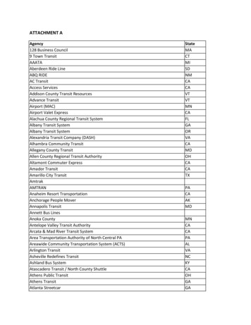
Chapter 09.01Golden Section Search MethodAfter reading this chapter, you should be able to:1.2.3.4.Understand the fundamentals of the Equal Interval Search methodUnderstand how the Golden Section Search method worksLearn about the Golden RatioSolve one-dimensional optimization problems using the Golden Section SearchmethodEqual Interval Search MethodOne of the simplest methods of finding the local maximum or local minimum is the EqualInterval Search method. Let’s restrict our discussion to finding the local maximum of f ( x )where the interval in which the local maximum occurs is [a, b] . As shown in Figure 1, let’schoose an interval of ε over which we assume the maximum occurs. Then we can compute a b ε a b ε a b ε a b ε . If f f , then the interval inf and f 2 2 2 2 2 2 2 2 a b ε a b ε which the maximum occurs is , b , otherwise it occurs in a, . This2 22 2 reduces the interval in which the local maximum occurs. This procedure can be repeated untilthe interval is reduced to the level of our choice.09.01.1

Golden Search Method09.01.2f(x)M M Aaεε22a b2BbxFigure 1A Equal interval search method (new upper bound can be identified).Remarks:As can be seen from the marked data points A, M , M , and B on Figure 1A, the functionvalues have increased from point A to point M-, but then have decreased from point M topoint M . Whenever there is a sudden change in the pattern, such as from increasing thefunction value to decreasing its value, as shown in Figure 1A (or vice versa, as shown inFigure 1B, where f L f 2 f1 and then f1 f u ), then the new lower and upper boundbracket values can be found. In this case, the new lower bound remains to be the same as itsprevious lower bound (at point A), and the new upper bound can be found (at point M ), asshown in Figure 1A.Figure 1B Equal interval search method (new lower bound can be identified).

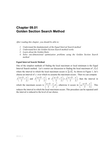
Golden Search Method09.01.3Example 1Consider Figure 2 below. The cross-sectional area A of a gutter with equal base and edgelength of 2 is given byA 4 sin θ (1 cos θ )Using an initial interval of [0, π / 2] , find the interval after 3 iterations. Use an initial intervalε 0.2 .2θ22θFigure 2 Cross section of the gutter.SolutionIf we assume the initial interval to be [0, π / 2] [0,1.5708] and choose ε 0.2 , then a b ε 0 1.5708 0.2 f f 2 22 2 f (0.88540 ) 5.0568 a b ε 0 1.5708 0.2 f f 2 22 2 f (0.6854) 4.4921Since f (0.88540 ) f (0.68540 ) , the interval in which the local maximum occurs is[0.68540,1.5708] .Now a b ε 0.68540 1.5708 0.2 f f 2 22 2 f (1.2281) 5.0334

Golden Search Method a b ε f 2 2 09.01.4 0.68540 1.5708 0.2 f 22 f (1.0281) 5.1942Since f (1.2281) f (1.0281) , the interval in which the local maximum occurs is[0.68540,1.2281] .Now a b ε 0.68540 1.2281 0.2 f f 2 22 2 f (1.0567 ) 5.1957 a b ε 0.68540 1.2281 0.2 f f 2 22 2 f (0.8567 ) 5.0025Since f (1.0567 ) f (0.8567 ) , then the interval in which the local maximum occurs is(0.8567,1.2281) . After sixteen iterations, the interval is reduced to 0.02 and theapproximation of the maximum area is 5.1961 at an angle of 60.06 degrees.The exact answer is θ 1.0472 for which f (θ ) 5.1962 .What is the Golden Section Search method used for and how does it work?The Golden Section Search method is used to find the maximum or minimum of a unimodalfunction. (A unimodal function contains only one minimum or maximum on the interval[a,b].) To make the discussion of the method simpler, let us assume that we are trying to findthe maximum of a function. The previously introduced Equal Interval Search method issomewhat inefficient because if the interval is a small number it can take a long time to findthe maximum of a function. To improve this efficiency, the Golden Section Search method issuggested.As shown in Figure 3, choose three points xl , x1 and xu ( xl x1 xu ) along the x-axis with corresponding values of the function f ( xl ) , f ( x1 ) , and f ( xu ) , respectively. Sincef (x1 ) f (xl ) and f (x1 ) f (xu ) , the maximum must lie between xl and xu . Now a fourthpoint denoted by x2 is chosen to be between the larger of the two intervals of [ xl , x1 ] and[ x1 , xu ] . Assuming that the interval [ xl , x1 ] is larger than [ x1 , xu ] , we would chose [ xl , x1 ] asthe interval in which x2 is chosen. If f (x2 ) f (x1 ) then the new three points would be

Golden Search Method09.01.5xl x2 x1 ; else if f (x2 ) f (x1 ) then the new three points are x2 x1 xu . This process iscontinued until the distance between the outer points is sufficiently small.f (x 2 )f (x )f (xl )f (x1)f(x )uxxxl2x1xuFigure 3 Cross section of the gutter.How are the intermediate points in the Golden Section Search determined?We chose the first intermediate point xl to equalize the ratio of the lengths as shown in Eq.(1) where a and b are distance as shown in Figure 4. Note that a b is equal to the distancebetween the lower and upper boundary points xl and xu .ab (1)a b af (x )f ( x1 )f ( xl )f ( xu )xxlax1 bxuFigure 4 Determining the first intermediate pointThe second intermediate point x2 is chosen similarly in the interval a to satisfy thefollowing ratio in Eq. (2) where the distances of a and b are shown in Figure 5.b a b ab(2)

Golden Search Method09.01.6f (x2 )f (x )f ( xl )f ( x1 )f ( xu )a-bbxlxax2x1xuFigure 5 Determining the second intermediate pointDoes the Golden Section Search have anything to do with the Golden Ratio?The ratios in Equations (1) and (2) are equal and have a special value known as the GoldenRatio. The Golden Ratio has been used since ancient times in various fields such asarchitecture, design, art and engineering. To determine the value of the Golden Ratio letR a / b , then Eq. (1) can be written as1 R or1RR2 R 1 0(3)Using the quadratic formula, the positive root of Eq. (3) is 1 1 4( 1)25 1 2 0.61803R (4)In other words, the intermediate points x1 and x2 are chosen such that, the ratio of thedistance from these points to the boundaries of the search region is equal to the golden ratioas shown in Figure 6.

Golden Search Method09.01.7f (x )f (x2 )f ( x1 )f ( xl )f ( xu )abxxlx2x1xuabFigure 6 Intermediate points and their relation to boundary pointsWhat happens after choosing the first two intermediate points?Next we determine a new and smaller interval where the maximum value of the function liesin. We know that the new interval is either [ xl , x 2 , x1 ] or [ x 2 , x1 , xu ] . To determine which ofthese intervals will be considered in the next iteration, the function is evaluated at theintermediate points x2 and x1 . If f ( x2 ) f ( x1 ) , then the new region of interest will be[ xl , x2 , x1 ] ; else if f ( x2 ) f ( x1 ) , then the new region of interest will be [ x2 , x1 , xu ] . InFigure 6, we see that f ( x2 ) f ( x1 ) , therefore our new region of interest is [ xl , x 2 , x1 ] . Weshould point out that the boundaries of the new smaller region are now determined by xl andx1 , and we already have one of the intermediate points, namely x2 , conveniently located at apoint where the ratio of the distance to the boundaries is the Golden Ratio. All that is left todo is to determine the location of the second intermediate point. Can you determine if thesecond point will be closer to xl or x1 ? This process of determining a new smaller region ofinterest and a new intermediate point will continue until the distance between the boundarypoints are sufficiently small.The Golden Section Search AlgorithmThe following algorithm can be used to determine the maximum of a function f (x) .Initialization:Determine xl and xu which is known to contain the maximum of the function f (x) .Step 1Determine two intermediate points x1 and x2 such that

Golden Search Method09.01.8x1 xl dwherex 2 xu dd 5 1( xu xl )2Step 2Evaluate f ( x1 ) and f ( x2 ) .If f ( x1 ) f ( x2 ) , then determine new xl , x1 , x2 and xu as shown in Equation set (5). Notethat the only new calculation is done to determine the new x1 .xl x 2x 2 x1(5)xu xu5 1( xu xl )2If f ( x1 ) f ( x2 ) , then determine new xl , x1 , x2 and xu as shown in Equation set (6). Notex1 xl that the only new calculation is done to determine the new x2 .xl xlxu x1(6)x1 x2x 2 xu 5 1( xu xl )2Step 3If xu xl ε (a sufficiently small number), then the maximum occurs atiterating, else go to Step 2.xu xland stop2Further Remarks and Explanation About The Golden Section Search AlgorithmThe above discussion has assumed that the user can determine x L and xu which is known tocontain the maximum of the function f (x) . In this section, the Golden Section algorithm isre-examined from a more rigorous viewpoint, and with the following 2 primary objectives:(a) Developing an automated procedure to determine the appropriated initial guesses forthe lower and upper bounds, respectively.

Golden Search Method09.01.9(b) Proving (in a more rigorous way) that we only needs to find/compute only 1 (not 2)intermediate point, based on the current bracket.To start the Golden Section search process, a small (positive) parameter “ δ ” is defined bythe user, say “ δ ” 0.05. The function value g( α δ ) g1 is initially computed. Thesecond interval will be 1.618 times the previous (or first) interval (or 1.618 * δ ), therefore,the next computed function value g( α 2.618 * δ ) g 2 is computed.Since g 2 is smaller than the previous value g1 [see Figure 6A], one continues to consider thethird interval which will be 1.618 times the second interval (or 1.618 * 1.618 δ 1.618 2 δ ),and the next computed function value g( α 5.232 * δ ) g 3 is computed. As indicated inFigure 6A, α (5.232 * δ ) is also labeled as the (j-2)-th point on the curve!Since g 3 is still smaller than the previous value g 2 [see Figure 6A], one continues toconsider the fourth interval which will be 1.618 times the third interval (or 1.618 * 1.618 2 δ 1.6183 δ and the next computed function value g ( α 9.468 * δ ) g 4 is computed. Asindicated in Figure 6A, α (9.468 * δ ) is also labeled as the (j-1)-th point on the curve!Since g 4 is still smaller than the previous value g 3 [see Figure 6A], one continues toconsider the fifth interval which will be 1.618 times the fourth interval (or 1.618 * 1.6183 δ 1.618 4 δ ), and the next computed function value g ( α 16.3215 * δ ) g 5 is computed. Asindicated in Figure 6A, α (16.3215 * δ ) is also labeled as the j-th point on the curve!At this moment, since g 5 g(at the j-th point) is larger than g 4 g(at the j-1-th point), the“decreasing pattern” is no longer true, therefore, we can establish the initial lower bound andthe initial upper bound to be equal to the values of α at the (j-2)-th location and at the j-thlocation, respectively !Based on the above observation and analysis, one can easily figure out the generalformulas to compute and identify the initial lower and upper bound values for α as indicatedin Figure 6A.Having found the initial lower and upper bounds for α , the 2 intermediate pointsα a and α b need be inserted (with the same distance measured from the lower bound andupper bound, respectively) as shown in Figure 6B. Using Figure 6B, α a can be computed anddisplayed as shown in equation (7).Finally, with trivial algebraic manipulations, the value for α a can be shown to be thesame as the value for α (at the j-1 th point), as indicated in equation (8).