Transcription
Asia-Pacific Finan Markets (2006) 13:235–258DOI 10.1007/s10690-007-9043-zOn a Non-linear Risk Analysis for Stock MarketIndexesKenjiro Suzuki · Yasunori Okabe · Takaaki FujiiPublished online: 19 July 2007 Springer Science Business Media, LLC 2007Abstract We propose a method to detect early signs of a potential major crashin the market from only the information of the time series representing its stockmarket data. As reinforcement of the abnormality test Test(ABN) developedin Okabe, Matsuura, and Klimek (International Journal of Pure and AppliedMathematics, 3, 443–484, 2002), we introduce in this paper a risk graph to measure abnormality of time series by using the non-linear prediction analysis inthe theory of KM2 O-Langevin equations. By applying it to real data of stockmarket indexes on the Black Monday of 1987 and those during the past 7 yearsfrom January 2000 to December 2006, we investigate whether we can detectearly signs of a potential major crash in the market by watching the behaviorof the risk graph.Keywords Stock market crashes · KM2 O-Langevin equation · Test(ABN) ·Abnormality graph · Stationarity graph · Risk graphK. Suzuki (B)Mitsubishi Research Institute Inc.,3-6, Otemachi 2-Chome, Chiyoda-ku, Tokyo, 100-8141, Japane-mail: ksuzuki@mri.co.jpY. Okabe · T. FujiiDepartment of Mathematical Informatics, Graduate School of Information Sicenceand Technology, University of Tokyo,Bunkyo-ku, Tokyo, 113-8656, Japane-mail: okabe@mist.i.u-tokyo.ac.jpT. Fujiie-mail: takaakifujii@mist.i.u-tokyo.ac.jp
236K. Suzuki et al.1 IntroductionThe central purpose of this paper is to propose a method to detect early signsof abnormality lurking behind a time series and to apply it to some time seriesin the Black Monday of 1987 and during the past 7 years from January 2000to December 2006 in financial market, by developing a non-linear risk analysisto reinforce the abnormality test Test(ABN) in the theory of KM2 O-Langevinequations.In financial time series analysis, the so called Value at Risk (VaR) is a standard method for measuring the market risk in the practical business. In the studyof VaR, “risk” is interpreted as the maximum loss of the assets concerned. Inconcrete, we regard all the trades as the derivative securities written on prices,rates or indexes observed in markets and the value of portofolio P(t) at presenttime t is given by a function of the prices of these original assets. Hence P(t)is a random variable because the original assets are all random variables. Ata certain time in the future t τ , if the phenomenon that the change of thevalue P P(t τ ) P(t) falls below a certain level X takes place withprobability α, then we call this X VaR at α.In general, there are three major methods for calculating VaR: delta method,Monte–Calro method, and Historical method. Delta method and Monte–Calromethod are used under the assumption that the earning ratios have the normaldistribution. However, many studies indicated that they often have distributions with fat-tail or larger coefficient of excess (Duffie and Pan, 1997). Fordealing with this problem, recently, Historical method attracts much attentionand many improved methods are proposed: BRW method including weightingfor data (Boudoukh et al., 1998), HW method and FHS method including nonlinear volatility estimation models (Barone-Adesi et al., 1999; Hull and White,1998). Their developments are expected for now owing to their better accuracy. However, we cannot ignor the inherent problem of Historical method thatshapes of distribution tend to be distorted when data number is small (Kupiec,1995).One of the aurthors (Matsuura and Okabe, 2001; Okabe and Kaneko, 2000)solved the non-linear prediction problem for discrete time stochastic processeswhich has been unsolved after Masani and Wiener’s work (Masani and Wiener,1959), by developing the theory of KM2 O-Langevin equations. Furthermore,he proposed in Okabe et al. (2002) a test for detecting early signs of abnormalityof time series in complex phenomena, to be called Test(ABN), based on thetheory of KM2 O-Langevin equations and applied it to historical financial indexdata at three major international market crashes in the economic history: TheBlack Monday of October 1987, Asian Crisis in mid-1997 and the collapse ofthe Internet Bubble in Spring 2000. In Okabe et al. (2002), he defines “normal condition” as “stationarity” and interpret “abnormality” as “rupture ofstationarity” in time series. The aim at Test(ABN) is to search the timing whenstationarity is lost, by applying the stationarity test Test(S) proposed in Okabeand Nakano (1991) to the non-linear transformed time series under investigation. The results of Test(ABN) are represented by the abnormality graph and
Risk Analysis for Stock Market Indexes237the stationarity graph. The former graph tells us when abnormality emerges interms of the collapse of stationarity and the latter graph tells us how the extentof stationarity breaks. If the stationarity graph begins to fall down after thepeak, we think that stationarity is breaking, namely, the abnormality is expanding. By examining these graphs carefully, we can acquire one guideline to graspthe signs of abnormality quantitatively. In fact, in Okabe et al. (2002), there areacquired certain accomplishment for detecting the early signs of some stockmarkets’ crashes.However, there remain some problems to be solved. One of them is thatthere emerge many time points where abnormality emerges or many time pointswhere the stationarity graph falls down, which we cannot distinguish them. Itprobably seems that abnormality of the time series cannot be expressed in termsof only the rupture of stationarity. This implies that it is needful to distinguishmany abnormality times which emerge globaly and then to catch certain globalfactors of abnormality.In order to overcome this problem, we meausre in this paper “risk” of timeseries by the prediction error and introduce the third risk graph of finite rankbesides the abnormality graph and the stationarity graph, by using non-linearprediction analysis in the theory of KM2 O-Langevin equations. The predictionerror stands for the extent of the separation between the real behavior and itsprediction. We can regard that the smaller the risk is, the more accurate theprediction is. By calculating the non-linear prediction error, we draw the riskgraph to catch certain global factors of abnormality quantitatively.We state the contents of this paper. In Sect. 2, we recall the non-linear prediction analysis in the theory of KM2 O-Langevin equations.In Sect. 3, we recall the abnormality test Test(ABN) and introduce a riskgraph associated with a time series. We give 13 steps for calculating three kindsof abnormality graph, stationarity graph and risk graph associated with a onedimensional time series Z (Z(n); 0 n N). We fix any L 1 (0 L N)to be called a cut length. We state the outline for defining a risk graph. First, forany fixed t (L t N), we extract a time series Z (t) (Z(n); t L n t) withterminal time t and length L 1. Next, by operating the non-linear transforma(t)tion of rank 6 to it, we construct 19 time series Zj (0 j 18). It is to notedthat Z0(t) Z (t) . Furthermore, by changing the time domain and taking the(t)standardization, we construct 18 two-dimensional time series X̃0j (1 j 18)(t)(t)whose first component and second componet are defined from Z0 and Zj ,respectively. Third, for any j(1 j 18) such that the time series X̃0j(t) satisfiesthe stationarity test Test(S), we calculate the sample covariance matrix function R(Z (t) , X̃0j(t) ) and obtain the linear prediction error PEj (Z; L)(t). Finally,we define a risk function RF(Z; L) RF(Z; L)(t) (L t N) by shifting theterminal time t. We call the graph of the risk function RF(Z; L) a risk graph ofcut length L 1 associated with the original time series Z.In Sect. 4, first, we present the results of experiments implemented for stockmarket indexes: Dow, Ftse 100, and Nikkei 225 in 1984–1988, which contains
238K. Suzuki et al.“Black Monday” on October 19, 1987. For each index, we show three kinds ofabnormality graph, stationarity graph and risk graph simultaneously. As statedin Okabe et al. (2002), the abnormality graphs show that there emerge manyabnormality times befor Black Monday. However, the risk graphs show thatthere exists a characteristic trend like the so-called V-shape in the period fromthe time right after PLaza Agreement on September 22, 1985 to the time justbefore Black Monday in the indexes, which implies that the risk graph can catchcertain global factors of abnormality of time series and reinforces Test(ABN).Next, we treat the same stock market indexes during the past 7 years from January 2000 to December 2006 and show that there appear certain interestingcharacteristic trends like the V-shape change in respective risk graphs.In Sect. 5, we review our results2 Non-linear Prediction AnalysisWe recall the non-linear prediction and filtering analysis in the theory ofKM2 O-Langevin equations: The former analysis was developed for onedimensional stochastic process in Matsuura and Okabe (2001) and extendedto multi-dimensional one in Okabe and Kaneko (2000), and the latter analysiswas developed for one-dimensional stochastic process in Okabe and Matsuura(2005).Let X (X(n); 0 n N) be any one-dimensional square integrable stochastic process defined on a probability space ( , B, P).[2.1] For any n1 , n2 (0 n1 n2 N), we define the non-linear informationspace Nnn21 (X) for the stochastic process X byNnn21 (X) {Y L2 ( , B, P); Y is a real-valued Bnn12 (X)-measurable function},(2.1)where Bnn12 (X) stands for the smallest σ -field with respect to which all randomvariables X(m) (n1 m n2 ) are measurable.Let {X(q) ; q N } be any generating system for the non-linear information spaces Nn0 (X) (0 n N) whose existence is proved in Okabe andMatsuura (2005), where N stands for the set of non-negative integers: EachX(q) (X (q) (n); 0 n N) is a d(q) -dimensional square integrable with meanvector 0 and(2.2)X(0) X,{X(q) ; q N } has a nest structure, that is,X (q 1) (n) Nn0 (X) X (q) (n), q N , 0 n N, n(q) {1}] [M0 (X ) ,q 0(2.3)0 n N,(2.4)
Risk Analysis for Stock Market Indexes239where for each n1 , n2 (0 n1 n2 N), the space Mnn21 (X(q) ) is the closedlinear information space defined by(q)Mnn21 (X(q) )2 {Y L ( , B, P); Y n2d (q)cjk Xj (k) (cjk R)}(2.5)j 1 k n1and for any subset S of L2 ( , B, P), [S] stands for the closed subspace ofL2 ( , B, P) which is generated by all elements in S.Fix any q N . Let R(X, X(q) ) (R(X, X(q) )(n, k); 0 n, k N) bethe covariance matrix function of the processes X and X(q) and R(X(q) ) (R(X(q) )(n, k); 0 n, k N) the covariance matrix function of the process X(q) :R(X, X(q) )(n, k) E(X(n)t X (q) (k))( M(1, d(q) ; R)),R(X(q) )(n, k) E(X (q) (n)t X (q) (k))( M(d(q) , d(q) ; R)).(2.6)(2.7)We note from (2.2) that R(X, X(q) )(n, k) is equal to the first row of R(X(q) )(n, k)(0 k n N).By (4.48) and (4.49) in Matsuura and Okabe (2001), we can describe thetime evolution of the process X(q) by the following forward KM2 O-Langevinequation:X (q) (0) ν (X(q) )(0),n 1 X (q) (n) (2.8)γ 0 (R(X(q) ))(n, k)X (q) (k) ν (X(q) )(n), 1 n N, (2.9)k 0where ν (X(q) ) (ν (X(q) )(n); 0 n N) is the forward KM2 O-Langevinfluctuation process and γ 0 (R(X(q) )) (γ 0 (R(X(q) ))(n, k); 0 k n N) theminimum forward KM2 O-Langevin dissipation matrix function associated withthe covariance matrix function R(X(q) ). Furthermore, we define the forwardKM2 O-Langevin fluctuation matrix function V (R(X(q) )) (V (R(X(q) ))(n); 0 n N) byV (R(X(q) ))(n) E(ν (X(q) )(n) t ν (X(q) )(n)).(2.10)We note that γ 0 (R(X(q) )) and V (R(X(q) )) can be calculated according to thegeneralized fluctuation–dissipation algorithm by using R(X(q) ) (Matsuura andOkabe, 2003; Okabe et al., 2002).For simplifying the notation, we put R(q) R(X, X(q) ). Furthermore, for anyw 0, we define a 1 d(q) matrix function R(q),w (R(q),w (n, k); 0 n, k N)and a d(q) d(q) matrix function R(q,w) (R(q,w) (n, k); 0 n, k N) byR(q),w (n, k) R(q) (n, k) w2 δnk ed(q) ,(q,w)R(q)(n, k) R(X2)(n, k) w δnk Id(q) ,(2.11)(2.12)
240K. Suzuki et al.where ed(q) (1, 0, . . . , 0) is the 1 d(q) matrix whose first element is 1 andothers are 0 and Id(q) is the d(q) d(q) identity matrix.Then we define a 1 d(q) matrix function C(R(q),w ) (C(R(q),w )(n, k); 0 k n N) byC(R(q),w )(n, k)R(q),w (n, 0)V (R(q,w) )(0) 1 ,k 0,k 1 (R(q),w (n, k) R(q),w (n, l) t γ (R(q,w) )(k, l))V (R(q,w) )(k) 1 , 1 k n,l 0(2.13)where the matrix function γ (R(q,w) ) (γ (R(q,w) )(k, l); 0 l k N)(respectively, V (R(q,w) ) (V (R(q,w) )(k); 0 k N)) is the forwardKM2 O-Langevin dissipation (respectively, fluctuation) matrix functionassociated with the positive-definite matrix function R(q,w) , respectively.By using (2.20) and Theorem 2.7 in Okabe and Matsuura (2005), we haveTheorem 2.1 (Okabe and Matsuura, 2005) For any n, k (0 k n N), thereexists a limit C0 (R(q) )(n, k) lim C(R(q),w )(n, k) andw 0PMn 1 (X(q) ) X(n) 0n 1 C0 (R(q) )(n, k)ν (X(q) )(k).k 0Furthermore, we see from (2.3) and (2.4) thatTheorem 2.2 (Matsuura and Okabe, 2001) (the non-linear prediction formula)For any n (1 n N)PNn 1 (X) X(n) lim0q n 1 E(X(n)) C0 (R(q) )(n, k)ν (X(q) )(k) .k 0[2.2] Next, we define the non-linear prediction error e(X)(n) and the nonlinear prediction error eq (X)(n) of rank q by 2 e(X)(n) E X(n) PNn 1 (X) X(n) ,0 2eq (X)(n) E X(n) E(X(n)) PMn 1 (X(q) ) X(n).(2.14)(2.15)0 By noting that eq (X)(n) E (X(n) E(X(n))) PMn 1 (X(q) ) (X(n) 0E(X(n))))2 , we see from Theorem 3.3 in Okabe and Yamane (1998) andTheorem 2.1 that
Risk Analysis for Stock Market Indexes241Theorem 2.3 (Okabe and Yamane, 1998) If t (X, X(q) ) is weakly stationary, thenfor any m, n(1 m n N)(1) 0 eq (X)(n) eq (X)(m) V(X)(0), 2(2) eq (X)(n) E X(N) E(X(N)) PMN 1 (X(q) ) X(N) ,(3) eq (X)(n) V(X)(0) Cn (X X(q) )2 ,N nwhere V(X)(0) E((X(0) E(X(0)))2 ) and Cn (X X(q) ) is given by Cn (X X(q) ) n 1 1/2C0 (R(q) )(n, k)V (X(q) )(k) t C0 (R(q) )(n, k) .k 0Finally, by Theorem 2.2, we haveTheorem 2.4 (Matsuura and Okabe, 2001) e(X)(n) limq eq (X)(n)(1 n N).3 Non-linear Risk Analysis for Time SeriesLet Z (Z(n); 0 n N) be any one-dimensional time series with lengthN 1. We recall the abnormality test Test(ABN) and state the procedure forobtaining the risk graph associated with the time series Z.Step 1 (cut length) Fix any two natural numbers L and t (1 L t N). Wedefine a time series Z (t) (Z (t) (n); 0 n L) with length L 1 byZ (t) (n) Z(n t L).(3.1)We note that Z (t) (L) Z(t). We call L 1 the cut length.Step 2 (standardization) By taking a standardization of the time series Z (t) ,we define a time series Z̃ (t) (Z̃ (t) (n); 0 n L) byZ̃ (t) (n) Z (t) (n) µ(Z (t) )υ(Z (t) ),(3.2)where µ(Z (t) ) and υ(Z (t) ) are the sample mean and the sample variance of thetime series Z (t) , respectively:µ(Z (t) ) 1 (t)Z (n),L 1(3.3)1 (t)(Z (n) µ(Z (t) ))2 .L 1(3.4)Ln 0υ(Z (t) ) Ln 0
242K. Suzuki et al.We note that the sample mean µ(Z̃ (t) ) and the sample variance υ(Z̃ (t) ) of thetime series Z̃ (t) are 0 and 1, respectively:µ(Z̃ (t) ) 0andυ(Z̃ (t) ) 1.(3.5)Step 3 (non-linear transformations of rank 6) By applying the non-lineartransformations of rank 6 to the time series Z̃ (t) , we construct 19 one(t)dimensional time series Zi (0 i 18) as follows:(t)Z0 (Z̃ (t) (n); 0 n L),(t)Z1 (Z̃ (t) (n)2 ; 0 n L),Z2(t) (Z̃ (t) (n)3 ; 0 n L),(t)Z3 (Z̃ (t) (n)Z̃ (t) (n 1); 1 n L),Z4(t) (Z̃ (t) (n)4 ; 0 n L),(t)Z5 (Z̃ (t) (n)2 Z̃ (t) (n 1); 1 n L),(t)Z6 (Z̃ (t) (n)3 Z̃ (t) (n 2); 2 n L),Z7(t) (Z̃ (t) (n)5 ; 0 n L),(t)Z8 (Z̃ (t) (n)3 Z̃ (t) (n 1); 1 n L),(t)Z9 (Z̃ (t) (n)2 Z̃ (t) (n 2); 2 n 7(t)Z18 (Z̃ (t) (n)Z̃ (t) (n 1)2 ; 1 (Z̃ (t) (n)Z̃ (t) (n 3); 3 (Z̃ (t) (n)6 ; 0 (Z̃ (t) (n)4 Z̃ (t) (n 1); 1 n L), (Z̃ (t) (n)3 Z̃ (t) (n 2); 2 n L), (Z̃ (t) (n)2 Z̃ (t) (n 1)2 ; 1(3.6) n L), n L), n L), n L), (Z̃ (t) (n)2 Z̃ (t) (n 3); 3 n L), (Z̃ (t) (n)Z̃ (t) (n 1)Z̃ (s) (n 2); 2 n L), (Z̃ (t) (n)Z̃ (t) (n 4); 4 n L).From here to Step 10, let i, j, k (0 i, j, k 18) be any fixed integers. We(t)denote by li the left-hand side of the time domain of the time series Zi :Zi(t) (Zi(t) (n); li n L).(t)(3.7)(t)We define a two-dimensional time series Zjk (Zjk (n); max{lj , lk } n L)by(t)(t)(t)Zjk (n) t (Zj (n), Zk (n)).(3.8)
Risk Analysis for Stock Market Indexes243(t)Step 4 (time change) By changing the time domain of the time series Zi andwe define a one-dimensional time series Xi(t) (Xi(t) (n); 0 n Li ) and(t),Zjk(t)(t)a two-dimensional time series Xjk (Xjk (n); 0 n Ljk ) byXi(t) (n) Zi(t) (n li ),(t)(3.9)(t)Xjk (n) Zjk (n max{lj , lk }),(3.10)where Li and Ljk are given byLi L li ,(3.11)Ljk L max{lj , lk }.(3.12)Step 5 (standardization) By taking the standardization of the one-dimen(t)sional time series Xi again, we define a one-dimensional time series(t)(t)X̃i (X̃i (n); 0 n Li ) byX̃i(t) (n) (t)(t)(t)Xi (n) µ(Xi ) ,(t)υ(Xi )(3.13)(t)where µ(Xi ) and υ(Xi ) are the sample mean and the sample variance of the(t)time series Xi , respectively. Furthermore, we define a two-dimensional time(t)(t)series X̃jk (X̃jk (n); 0 n Ljk ) by(t)(t)(t)X̃jk (n) t (X̃j (n), X̃k (n)).(3.14)Step 6 (sample covariance matrix functions) We define a sample covariance(t)(t)matrix function R(X̃i ) (R(X̃i )(n); n Li ) of the one-dimensional time(t)series X̃i by(t)R(X̃i )(n) (t)R(X̃i )( n)L i n1X̃i(t) (n l)t X̃i(t) (l),Li 1 l 0(t)R(X̃i )(n),0 n Li ,(3.15)0 n Li(t)(t)and a sample covariance matrix function R(X̃jk ) (R(X̃jk )(n); n Ljk ) of(t)the two-dimensional time series X̃jk by(t)L nR(X̃jk )(n) (t)R(X̃jk )( n)jk 1(t)(t)X̃jk (n l)t X̃jk (l),Ljk 1 l 0t R(X̃ (t) )(n),jk0 n Ljk ,0 n Ljk .(3.16)
244K. Suzuki et al.(t)It is to be noted that the sample covariance function R(X̃i ) and the samplecovariance matrix function R(X̃jk(t) ) are all non-negative definite (Okabe andNakano, 1991).Step 7 (sample KM2 O-Langevin matrices) Therefore, according to thegeneralized fluctuation–dissipation algorithm (Matsuura and Okabe, 2003;(t)Okabe et al., 2002), we can construct the system LM(R(X̃i )) of the minimum(t)KM2 O-Langevin matrices associated with the function R(X̃i ) and the system(t)LM(R(X̃jk )) of the minimum KM2 O-Langevin matrices associated with the(t)matrix function R(X̃jk ): LM(R(X̃i(t) )) γi(t),0 (n, l), δi(t),0 (n), Vi(t) (m); 0 l n Li , 0 leq m Li , (3.17) (t)(t),0(t),0(t)LM(R(X̃jk )) γjk (n, l), δjk (n), Vjk (m); 0 l n Ljk , 0 m Ljk .(3.18)(t)We note that the elements of the system LM(R(X̃i )) and the systemLM(R(X̃jk(t) )) are real numbers and 2 2 matrices, respectively.Step 8 (sample KM2 O-Langevin equations) By using the elements of the(t)system LM(R(X̃i )), we derive the forward sample KM2 O-Langevin equationfor the time series X̃i(t) :X̃i(t) (n) n 1 γi(t) (n, l)X̃i(t) (l) ν (X̃i(t) )(n),(3.19)l 0(t)(t)where ν (X̃i ) (ν (X̃i )(n); 0 n Li ) is the one-dimensional(t)KM2 O-Langevin fluctuation time series associated with the time series X̃i .Similarly, we derive the forward sample KM2 O-Langevin equation for the(t)time series X̃jk :(t)X̃jk (n) n 1 (t)(t)(t)γjk (n, l)X̃jk (l) ν (X̃jk )(n),(3.20)l 0(t)(t)where ν (X̃jk ) (ν (X̃jk )(n); 0 n Ljk ) is the two-dimensional(t)KM2 O-Langevin fluctuation time series associated with the time series X̃jk .Step 9 (fluctuation–dissipation principle) We define a one-dimensional timeseries ξ(X̃i(t) ) (ξ(X̃i(t) )(n); 0 n Li ) and a two-dimensional time series(t)(t)ξ(X̃jk ) (ξ(X̃jk )(n); 0 n Ljk ) byν(X̃i(t) )(n) Wi(t) (n)ξ(X̃i(t) )(n),(3.21)(t)ν(X̃jk )(n)(3.22) (t)(t)Wjk (n)ξ(X̃jk )(n),
Risk Analysis for Stock Market Indexes(t)245(t)(t)where Wi (n) and Wjk (n) stand for the square root of the real number Vi (n)(t)(n), respectively.and the matrix VjkAccording to the fluctuation–dissipation principle (FDP) (Matsuura andOkabe, 2003; Okabe et al., 2002), we find that the one-dimensional (respec(t)(t)tively, two-dimensional) time series X̃i (respectively, X̃jk ) is a realization ofa one-dimensional (respectively, two-dimensional) weakly stationary process(t)(t)with R(X̃i ) (respectively, R(X̃jk )) as its covariance function (respectively,covariance matrix function) if and only if the one-dimensional time series(respectively, two-dimensional) ξ(X̃i(t) ) (respectively, ξ(X̃jk(t) )) is a realizationof a one-dimensional (respectively, two-dimensional) weakly white noise.As described in Okabe et al. (2002) and Okabe and Nakano (1991), by usingthe central limit theorem and the law of large numbers, we can obtain statisticalcriteria for the following three tests Test(M), Test(V), and Test(O) for the abovestatement for the one-dimensional time series X̃i(t) :(t)Test(M) : µ(ξ(X̃i )) 0,(t)Test(V) : υ(ξ(X̃i )) 1,(t)Test(O) : R(ξ(X̃i ))(n) 0 (1 n Li ),(t)(t)(t)where µ(ξ(X̃i )), υ(ξ(X̃i )) and R(ξ(X̃i )) is the sample mean, the sample variance and the sample covariance function of the time series ξ(X̃i(t) ), respectively.Similarly, we can give statistical criteria for the following three tests Test(M),Test(V), and Test(O) for the statement in the FDP for the two-dimensional(t)time series X̃jk :(t)Test(M) : µ(ξ(X̃jk )) 0,(t)Test(V) : υ(ξ(X̃jk )) t (1, 1),Test(O) : R(ξ(X̃jk(t) ))(n) 0 (1 n Ljk ),(t)(t)(t)where µ(ξ(X̃jk )), υ(ξ(X̃jk )), and R(ξ(X̃jk )) is the sample mean vector, thesample variance vector and the sample covariance matrix function of the timeseries ξ(X̃jk(t) ), respectively.Step 10 (Test(S)) By noting that a reliable number of the sample covari(t)ance function R(X̃i ) is at most 1 Mi [ 3(Li 1)], for each s (0 s (t)Li Mi ), we shift the starting time of the time series X̃i to get a time series(t),s(t)(t)X̃i (X̃i (n s); 0 n Mi ) with initial value X̃i (s) and derive a one(t),s(t),sby usingdimensional time series ξ(X̃i ) associated with the time series X̃i(t) (relia):the same system LM(R(X̃i )) LM(R(X̃i(t) ))(relia) γi(t),0 (n, l), δi(t),0 (n), Vi(t) (m); 0 l n Mi , 0 m Mi .(3.23)
246K. Suzuki et al.(t)We say that the time series X̃i satisfies Test(S) if the rate of s (0 s Li Mi )(t),sfor which Test(M), Test(V), and Test(O) for the time series ξ(X̃i ) holds ismore than or equal to 80, 70, and 80%, respectively.Next, we reduce the procedure to check the statistical criteria for Test(M),Test(V), and Test(O) for the two-dimsensional case to those for one-dimensional case. By noting that a reliable number of the sample covariance matrix(t)function R(X̃jk ) is at most 1 Mjk [ 3(Ljk 1)/2], for each s (0 s Ljk Mjk ), we derive a two-dimensional time series ξ(X̃jk(t),s ) associated with(t),sthe time series X̃jk(t)by using the system LM(R(X̃jk ))(relia) : (t),0(t),0(t)LM(R(X̃jk(t) ))(relia) γjk (n, l), δjk (n), Vjk (m); 0 l n Mjk , 0 m Mjk .(3.24)(t),sFurthermore, we arrange two components of the time series ξ(X̃jk ) into arow to get a one-dimensional time series ξ̇ (X̃jk(t),s ) with length 2(Mjk 1). We(t)say that the time series X̃jk satisfies Test(S) if two one-dimensional time series(t)(t)X̃j and X̃k satisfy Test(S), and moreover the rate of s (0 s Ljk Mjk )for which Test(M), Test(V), and Test(O) for the one-dimensional time seriesξ̇ (X̃jk(t),s ) holds is more than or equal to 80, 70, and 80%, respectively.Step 11 (Test(ABN) We recall Test(ABN) that detects early signs of abnormalbehavior of the one-dimensional time series Z (Z(n); 0 n N).We define an stationarity function ST(Z; L) : {L, L 1, . . . , N} [0, )by(t)ST(Z; L)(t) the number of two-dimensional time series X̃jk (0 j k 18)satisfying Test(S).(3.25)We say that there exists a sign of abnormality at time t (L 1 t N)for the time series Z if ST(Z; L)(t 1) 1 and ST(Z; L)(t) 0. We call thegraph of the function ST(Z; L) the stationarity graph associated with the timeseries Z and cut length L 1. Moreover, we define the abnormality graph byindicating the chart of the real data under investigation and the period whereST(Z; L)(t) 0 by the solid line and and black shaded areas, respectively.Step 12 (sample covariance matrix functions) From this step to the next step,we define a risk graph associated with the time series Z.Similarly as in Step 1, fix any two natural numbers L and t (1 L t N). For(t)any j (1 j 18) such that the time series X̃0j satisfies Test(S) in Step 10, we de(t)(t)fine a sample covariance matrix function R(Z (t) , X̃0j ) (R(Z (t) , X̃0j )(n); n L0j ) between the one-dimensional time series Z (t) and the two-dimensional(t)time series X̃0j by
Risk Analysis for Stock Market Indexes(t)R(Z (t) , X̃0j )(n)247L0j n 1(t) Z (t) (n l)t X̃0j (l),L0j 1(t)R(Z (t) , X̃0j )( n) l 0t R(Z (t) , X̃ (t) )(n),0j0 n L0j ,(3.26)0 n L0j .We note that Z (t) defined in (3.1) is not standardized, whereas X̃0j(t) is done.Furthermore, it is to be noted that reliable number of the sample covariance(t)matrix function R(Z (t) , X̃0j ) is at most 1 N0j [ 3(L0j 1)/3].(t)Step 13 (risk graph) Since the time series X̃0j satisfies Test(S), we find that(t)the time series Z (t) and X̃0j is a realization of a weakly stationary processX(t) (X (t) (n); 0 n L0j ) with covariance function given by the (1, 1)-com(t)ponent of R(Z (t) , X̃0j(t) ) and a weakly stationary process X̃(t)0j (X̃0j (n); 0 n (t)L0j ) with covariance matrix function given by R(X̃0j ), respectively.By applying the processes X, X(q) and the natural numbers n, N in thenon-linear prediction error eq (X)(n) of rank q in Theorem 2.3(2) to the(t)and the natural numbers N0j , L0j , respectively, we defineprocesses X(t) , X̃0ja prediction error PEj (Z; L)(t) byPEj (Z; L)(t) the first component of υ(t (Z (t) , t X̃0j(t) )) CN0j (Z (t) X̃0j(t) )2 ,(3.27)(t)where υ(t (Z (t) , t X̃0j )) is the sample variance vector of the three-dimensional(t)time series t (Z (t) , t X̃0j ) and (t)Cn (Z (t) X̃0j ) n 1 1/2(t)(t)(t)C0 (R(Z (t) , X̃0j ))(n, k)V0j (k)t C0 (R(Z (t) , X̃0j ))(n, k) ,k 0(3.28)(t)where C0 (R(Z (t) , X̃0j ))(n, k) is the 1 2 matrix function given by replacing(t)R(q) R(X, X(q) ) in Theorem 2.1 by the 1 2 matrix function R(Z (t) , X̃0j ).After the above preparations, we define a function RF(Z; L) : {L, L 1, . . . , N} [0, ) by (t)RF(Z; L)(t) min PEj (Z; L)(t); the time series X̃0j (1 j 18) satisfy Test(S) .(3.29)We call it the risk function associated with the time series Z and call the graphof the risk function RF(Z; L) a risk graph.
248K. Suzuki et al.Black Monday2600Dow2200180014001000Jan 84Jan 852400Ftse100Jan 86Jan 87Jan 88Jan 89Black Monday200016001200800Jan 84Jan 85Jan 86Jan 87Jan 88Jan 89Black Monday28000Nikkei225240002000016000120008000Jan 84Jan 85Jan 86Jan 87Jan 88Jan 89Fig. 1 Stock market indexes4 Results of Empirical Analyses for Stock Market Indexes4.1 Period: January 1984 – December 1988In this section, we apply the non-linear risk analysis introduced in Sect. 3 tostock market indexes of Dow Jones Industrial Averages (abbrev. Dow) from US,100-issue Ftse Average (abbrev. Ftse 100) from UK and 225-issue Nikkei Average (abbrev. Nikkei 225) from Japan in the period January 1984 – December1988 containing a major financial breakdown: Black Monday. Figure 1 shows theadjusted daily closed price data of Dow, Ftse 100, and Nikkei 225 in 1984–1988.These data were provided by www.Blomberg.com. We took N 1263, 1198,and 1224 for them, respectively.Here we recall the public recognition about Black Monday. It is ever largestscale fall in stock prices in New York, which occurred on Monday October 19,1987. On Black Monday, Dow Jones fell by as much as 508 a day, the fallingdown ratio was 23.8%. The stock falling ran over immediately and damagedinnumerable investors in the world. It is said that people got into a panic andterrified at the rumor of breaking out of the war.There are many explanations concerning probable causes concerning thecrash, particularly in the United States. According to some experts, it is said tobe a result of Plaza Agreement on September 22, 1985. For taking measures
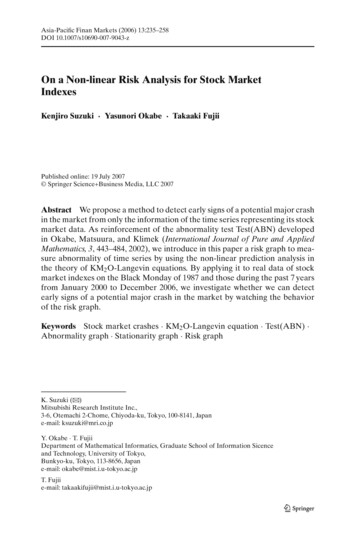
Risk Analysis for Stock Market Indexes249Black MondayBlack Monday2600160DowDow220080180014001000Jan 84Jan 85Jan 86Jan 87Jan 88Jan 890Jan 84Jan 85Jan 86Jan 87Jan 88Jan 89Black Monday0.5Dow0.40.30.20.10Jan 84Jan 85Jan 86Jan 87Jan 88Jan 89Fig. 2 Dow jones: Test(ABN) and risk graphto meet the excessive strong dollar, US held a meeting where the Ministers ofFinances and the Governors of the central banks from five advanced nations(G5) attended. At the meeting, the participating nations agreed to make theircurrencies to be devalued for 10–12% per the dollar by their “harmonious intervention”. They say that, as a result, the price of the dollar fell down rapidly andthe structure of economy and industry of US lost its balance (Bloomfield andO’hara, 1999). Other experts say that pricing of the stock market index futureswritten on the Standard and Poors Index stopped reflecting the value of thestocks used in the calculation of that index. As another factor, it is said thatthe trading systems used by institutional investors in US were programmed totrade automatically without any relation to their will, therefore too many sellingorders rushed. A variety of other factors have also been suggested: Bad practices in the money world, the l
By applying it to real data of stock market indexes on the Black Monday of 1987 and those during the past 7years from January 2000 to December 2006, we investigate whether we can detect early signs of a potential major crash in the market by watching the behavior of the risk graph. Keywords Stock market cra